Why R Markdown?
Overview
Teaching: 15 min
Exercises: 5 minQuestions
What is reproducible research?
How can R Markdown help research to be more reproducible?
What are the benefits of using R Markdown?
Objectives
Understand what scientific reproducibility entails.
Identify the benefits of using R Markdown to create research reports.
Understand how R Markdown is a useful tool in Open Science approaches.
Learn how R Markdown can help one’s research.
Warm-up
Let’s get into breakout rooms. What is reproducibility for you? Have you ever experienced issues to reproduce someone else’s study or even your own research?
The importance of Reproducibility in Research
Discussion: A scary anecdote
- A group of researchers obtain great results and submit their work to a high-profile journal.
- Reviewers ask for new figures and additional analysis.
- The researchers start working on revisions and generate modified figures, but find inconsistencies with old figures.
- The researchers can’t find some of the data they used to generate the original results, and can’t figure out which parameters they used when running their analyses.
- The manuscript is still languishing in the drawer…
According to the U.S. National Science Foundation (NSF) subcommittee on replicability in science:
Science should routinely evaluate the reproducibility of findings that enjoy a prominent role in the published literature. To make reproduction possible, efficient, and informative, researchers should sufficiently document the details of the procedures used to collect data, to convert observations into analyzable data, and to analyze data.
Reproducibility refers to the ability of a researcher to duplicate the results of a prior study using the same materials as were used by the original investigator. That is, a second researcher might use the same raw data to build the same analysis files and implement the same statistical analysis in an attempt to yield the same results. Reproducibility is a minimum necessary condition for a finding to be considered rigorous, believable and informative.
Why all the talk about reproducible research?
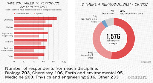
A 2016 survey in Nature revealed that irreproducible experiments are a problem across all domains of science:
Factors behind irreproducible research
- Not enough documentation on how experiment is conducted and data is generated
- Data used to generate original results unavailable
- Software used to generate original results unavailable
- Difficult to recreate software environment (libraries, versions) used to generate original results
- Difficult to rerun the computational steps
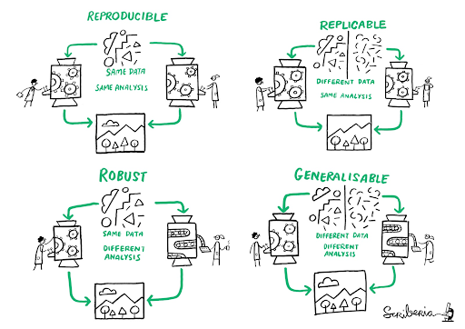
Reproducible, replicable, robust, generalizable
While reproducibility is the minimum requirement and can be solved with “good enough” computational practices, replicability/robustness/generalizability of scientific findings are an even greater concern involving research misconduct, questionable research practices (p-hacking, HARKing, cherry-picking), sloppy methods, and other conscious and unconscious biases.
If contributing to science and other researchers seems not to be compelling enough, here are 5 selfish reasons to work reproducibly (Markowetz, 2015)
- Helps to avoid data loss and disaster
- Makes it easier to write papers
- Helps reviewers see it your way
- Enables continuity of your work
- Helps to build your reputation
When do you need to worry about reproducibility?
Let’s assume that I have convinced you that reproducibility and transparency are in your own best interest. Then what is the best time to worry about it?
Throughout the whole research life cycle! Before you start the project because you might have to learn tools like R or Git. While you do the analysis because if you wait too long you might lose a lot of time trying to remember what you did two months ago. When you write the paper because you want your numbers, tables, and figures to be up-to-date. When you co-author a paper, because you want to make sure that the analyses presented in a paper with your name on are sound. When you review a paper, because you can’t judge the results if you don’t know how the authors got there.
Levels of Reproducibility
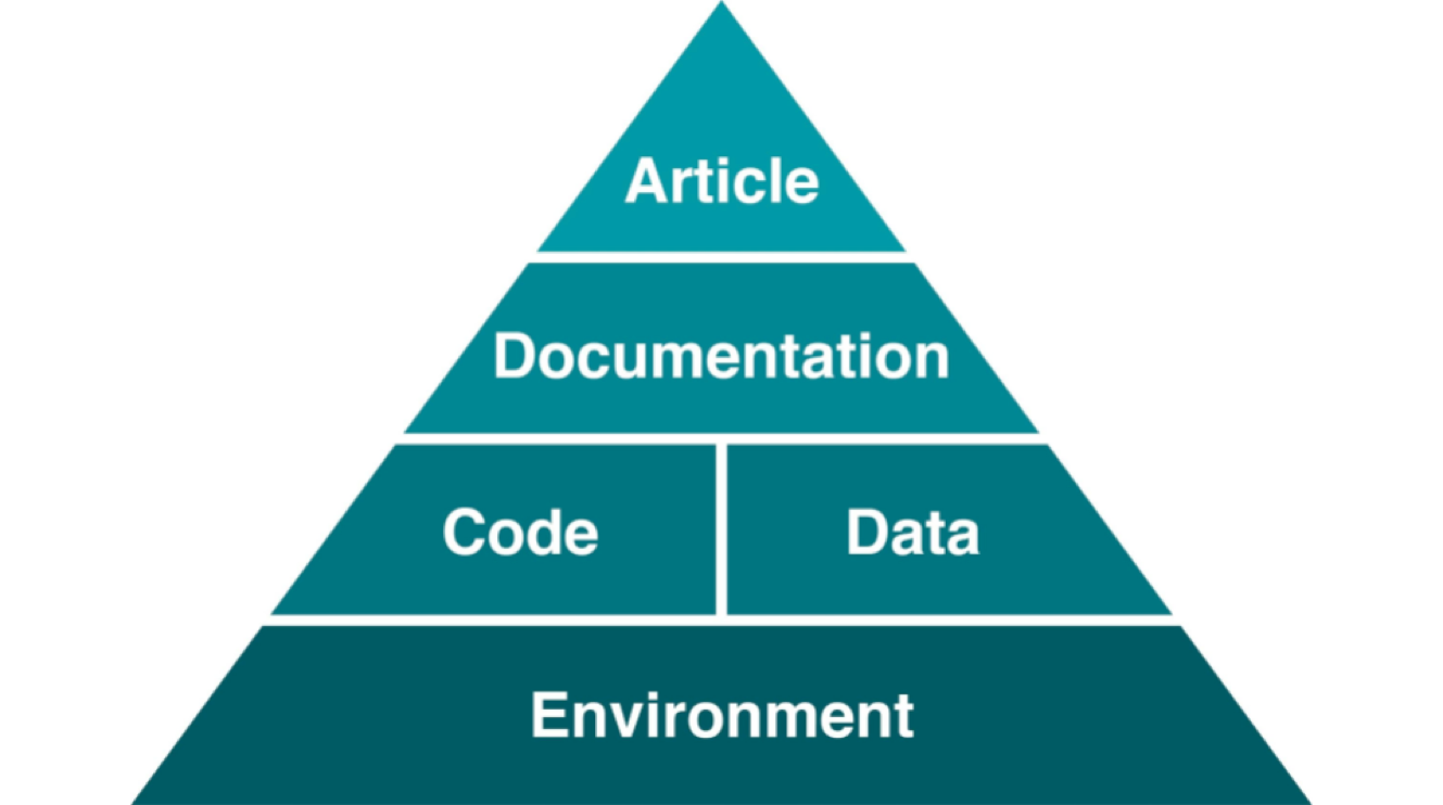
A published article is like the top of a pyramid, meaning that a reproducible paper/report rests on multiple levels that each contributes to its reproducibility.
What is R Markdown and how it connects to reproducible research?
R Markdown is a variant of Markdown, a system for writing simple, readable text that is easily converted to html which allows you to write using an easy-to-read, easy-to-write plain text format.
R Markdown belongs to the field of literate programming which is about weaving text and source code into a single document to make it easy to create reproducible web-based reports. Markdown is a simple formatting syntax for authoring HTML, PDF, and MS Word documents and much, much more. R Markdown provides the flexibility of Markdown with the implementation of R input and output. For more details on using R Markdown check http://rmarkdown.rstudio.com.
The idea of literate programming shines some light on this dark area of science. This is an idea from Donald Knuth where you combine your text with your code output to create a document. This is a blend of your literature (text), and your programming (code), to create something that you can read from top to bottom. Imagine your paper - the introduction, methods, results, discussion, and conclusion, and all the bits of code that make each section. With R Markdown, you can see all the pieces of your data analysis altogether.
You can include both text and code to execute. It is a convenient tool for reproducible and dynamic reports with R! With R Markdown, you are able to:
- Keep an eye on text (the paper) AND the source code. These computational steps are essential to ensure computational reproducibility.
- Conduct the entire analysis pipeline in an R Markdown document: data (pre-)processing, analysis, outputs, visualization.
- Apply a formatting syntax that is part of the R ecosystem and supports LaTeX.
- Combine text written in Markdown and source code written in R (and other languages).
- Easily share R Markdown documents with colleagues, as supplemental material, or as the paper under review. Thanks to the package knitr, others can execute the document with a single click and receive, for example, HTML or PDF renderings.
- Get figures automatically updated if you change the underlying parameters in the code. The error-prone task of exporting figures and uploading the right figure version to another platform is thus not needed anymore.
- Since Markdown is a text-based format, you can also use versioning control with Git.
- If you do not make any changes to the document after creating the output document, you can be sure that the paper was executable at least at the time of submission.
- Refer to the corresponding code lines in the methodology section making it unnecessary to use pseudocode, high-level textual descriptions, or just too many words to describe the computational analysis.
- Use packages such as rticles to use templates from publishers and create submission-ready documents.
Some Real-world Applications
Finally, three real-world examples that motivated the authors of this lesson to value and use R Markdown:
-
In the early days of the COVID-19 pandemic ecologist Chris Lortie quickly put together a simple but compelling COVID trends page. The ease with which he created his plots is a testament to the power of R as a data analysis environment, but the ease with which he was able to publish a page on the web is a testament to R Markdown and Github as a publishing environment. Notice that he did not have to: create plots in a tool and then export the plots as images; write any HTML; embed plot images in HTML; or create a site under Wordpress or other web hosting service. Instead, he directly published his R code as he wrote it, and using Github, made it appear on the web with a button click.
-
One of us wanted to create a short document that included some math formulas. The LaTeX document preparation can be used for this, but it is difficult to use and is overkill for just a few formulas in otherwise plain text. R Markdown lets you use just the best part of LaTeX—math formatting—while letting you write your text in a user-friendly way.
-
In this lesson we will be constructing a scientific paper that is based on an actual Nature publication and attendant survey and data. In trying to recreate the plots the original authors created, we found it difficult and time-consuming to figure out exactly how the authors created their plots. Out of the many columns in their data, many with similar-sounding names, which did they use? How did they handle missing data? Exactly what operations did they perform to compute aggregate values? How much easier it would have been if they had published the code they used along with their paper. R Markdown allows you to do this.
Our goal is that by the end of this workshop you will be able to create a reproducible report applying R Markdown and Knitr to publish a paper such as this example. This template is used exclusively for instruction purposes and is based on short and adapted version of the following academic paper:
Knudtson, K. L., Carnahan, R. H., Hegstad-Davies, R. L., Fisher, N. C., Hicks, B., Lopez, P. A., ... & Sol-Church, K. (2019). Survey on scientific shared resource rigor and reproducibility. Journal of biomolecular techniques: JBT, 30(3), 36. doi: doi: 10.7171/jbt.19-3003-001
Key Points
Reproducible research is key for scientific advancement.
R Markdown can help you to organize, have better control over and produce reproducible research.
Getting Started with R Markdown
Overview
Teaching: 15 min
Exercises: 10 minQuestions
How to find your way around RStudio?
How to start an R Markdown document in Rstudio?
How is an R Markdown document configured & what is our workflow?
Objectives
Key Functions in Rstudio
Learn how to start an R markdown document
Understand the workflow of an R Markdown file
Getting Around RStudio
Throughout this lesson, we’re going to teach you some of the fundamentals of using R Markdown as part of your RStudio workflow.
We’ll be using RStudio: a free, open source R Integrated Development Environment (IDE). It provides a built in editor, works on all platforms (including on servers) and provides many advantages such as integration with version control and project management.
This lesson assumes you already have a basic understanding of R and RStudio but we will do a brief tour of the IDE, review R projects and the best practices for organizing your work, and how to install packages you may want to use to work with R Markdown.
Basic layout
When you first open RStudio, you will be greeted by three panels:
- The interactive R console/Terminal (entire left)
- Environment/History/Connections (tabbed in upper right)
- Files/Plots/Packages/Help/Viewer (tabbed in lower right)
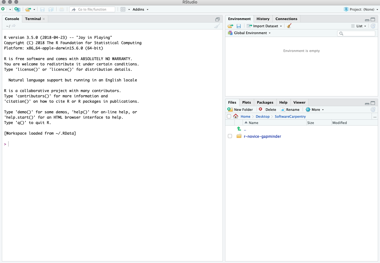
Once you open files, such as .Rmd files or .R files, an editor panel will also open in the top left.
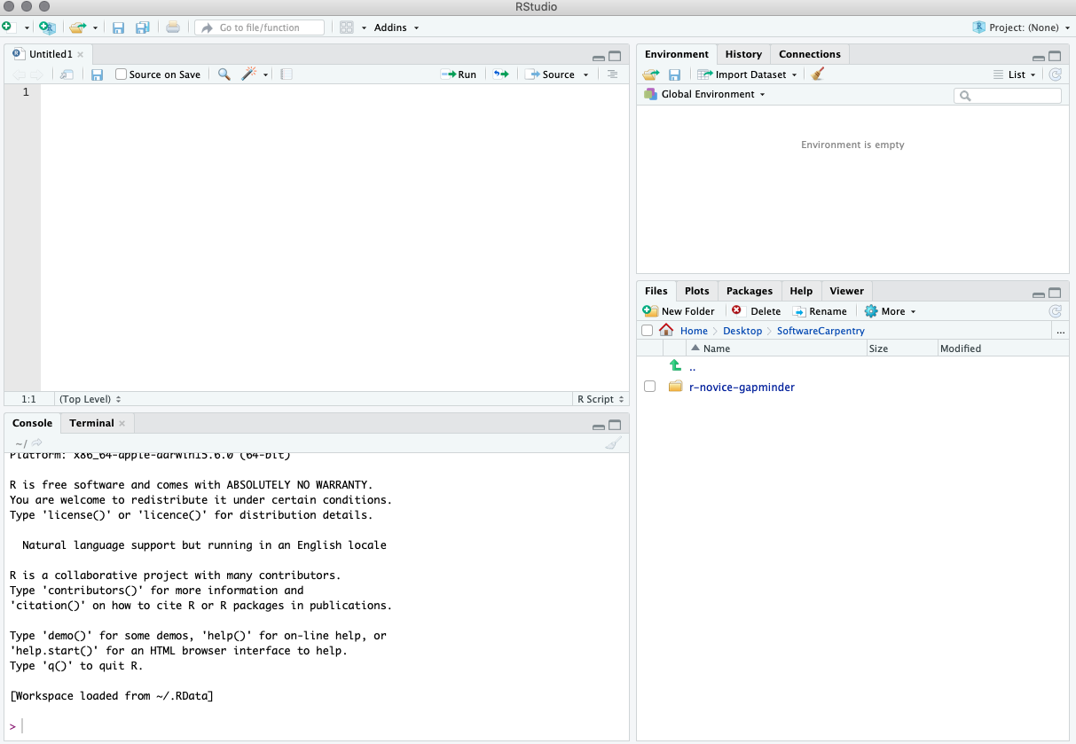
Working in an R Project
The scientific process is naturally incremental, and many projects start life as random notes, some code, then a manuscript, and eventually everything is a bit mixed together.
Managing your projects in a reproducible fashion doesn't just make your science reproducible, it makes your life easier.
— Vince Buffalo (@vsbuffalo) April 15, 2013
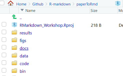
Most people tend not to think about how to organize their files which may result in something like this:
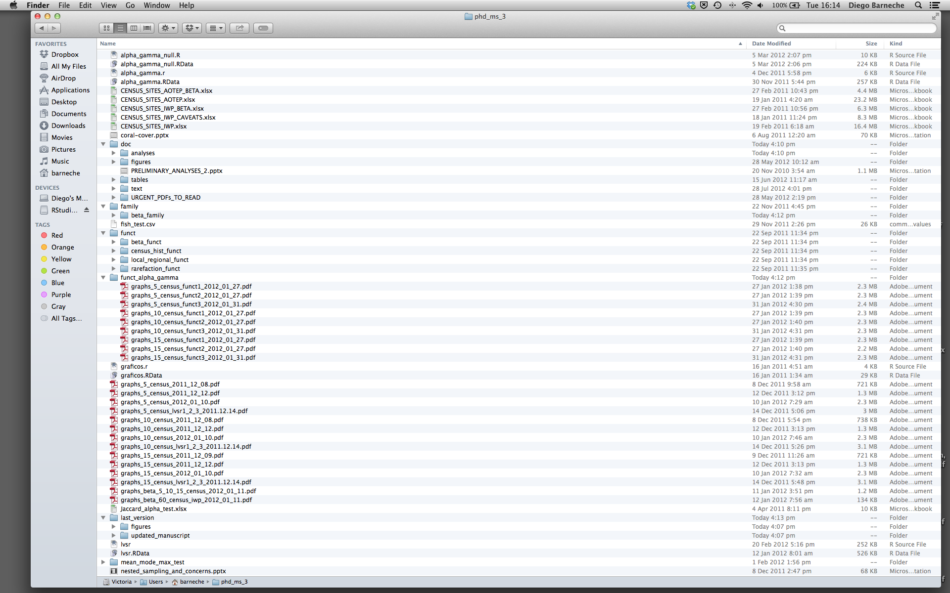
There are many reasons why we should ALWAYS avoid this:
- It is really hard to tell which version of your data is the original and which is the modified;
- It gets really messy because it mixes files with various extensions together;
- It probably takes you a lot of time to actually find things, and relate the correct figures to the exact code that has been used to generate it;
A good project layout will ultimately make your life easier:
- It will help ensure the integrity of your data;
- It makes it simpler to share your code with someone else (a lab-mate, collaborator, or supervisor);
- It allows you to easily upload your code with your manuscript submission;
- It makes it easier to pick the project back up after a break.
A possible solution
Fortunately, there are tools and packages which can help you manage your work effectively.
One of the most powerful and useful aspects of RStudio is its project management functionality. We’ll be using an R project today to complement our R Markdown document and bundle all the files needed for our paper into a self-contained, reproducible project. After opening the project we’ll review good ways to organize your work.
The simplest way to open an RStudio project once it has been created is to click
through your file system to get to the directory where it was saved and double
click on the .Rproj file. This will open RStudio and start your R session in the
same directory as the .Rproj file. All your data, plots and scripts will now be
relative to the project directory. RStudio projects have the added benefit of
allowing you to open multiple projects at the same time each open to its own
project directory. This allows you to keep multiple projects open without them
interfering with each other.
CHALLENGE 2.1 - Opening a Project in RStudio
Open an RStudio project through the file system
- Exit RStudio.
- Navigate to the directory where you downloaded & unzipped the zip folder for this workshop
- Double click on the
.Rprojfile in that directory.SOLUTION
double click on the
RMarkdown_Workshop.Rprojto automatically open in R Studio
Best practices for project organization
Although there is no “best” way to lay out a project, there are some general principles to adhere to that will make project management easier:
Treat data as read only
This is probably the most important goal of setting up a project. Data is typically time consuming and/or expensive to collect. Working with them interactively (e.g., in Excel) where they can be modified means you are never sure of where the data came from, or how it has been modified since collection. It is therefore a good idea to treat your data as “read-only”.
Data Cleaning
In many cases your data will be “dirty”: it will need significant preprocessing to get into a format R (or any other programming language) will find useful. This task is sometimes called “data munging”. Storing these scripts in a separate folder, and creating a second “read-only” data folder to hold the “cleaned” data sets can prevent confusion between the two sets.
Treat generated output as disposable
Anything generated by your scripts should be treated as disposable: it should all be able to be regenerated from your scripts.
There are lots of different ways to manage this output. Having an output folder with different sub-directories for each separate analysis makes it easier later. Since many analyses are exploratory and don’t end up being used in the final project, and some of the analyses get shared between projects.
Use Rmd files to combine code/analysis and narrative
Rmd combines the power of R code and analysis with narratives describing methods and results. Keeping your code and narrative in the same document increases reproducibility by bundling paper components together; decreasing the amount of work you, your collaborators, and your audience has to do to search for different components of your project: raw data, analysis and plots, narrative, and citations.
Tip: Good Enough Practices for Scientific Computing
Good Enough Practices for Scientific Computing gives the following recommendations for project organization:
- Put each project in its own directory, which is named after the project.
- Put text documents associated with the project in the
docdirectory.- Put raw data and metadata in the
datadirectory, and files generated during cleanup and analysis in aresultsdirectory.- Put source for the project’s scripts and programs in the
srcdirectory, and programs brought in from elsewhere or compiled locally in thebindirectory.- Name all files to reflect their content or function.
For this project, we used the following setup for folders and files:
bin: contains a a .csl file for changing the bibliography to APA format
code: a different name for the src folder. This will contain our R scripts for plots and R Markdown scripts for writing our paper.
data: this folder contains our raw data files. We have 3 .csvs
docs: This contains our raw text file paper_raw.txt for the paper and our bibliography.bibtex for reference. We could add any other notes we may have about the project here too.
figs: This is for the .png figures we found and want to add into our paper. It can also be used to save .png or .jpeg copies of the figures we output from our code.
results: This is where the rendered version of our .Rmd file (and .R scripts if we ran them) will save to in html form.
RMarkdown_Workshop.Rproj lives in the root directory.
Optional Files to add to root directory:
README.md A detailed project description with all collaborators listed.
CITATION.txt Directions to cite the project.
LICENSE.txt Instructions on how the project or any components can be reused.
Again, there are no hard and fast rules here, but remember, it is important at least to keep your raw data files separate and to make sure they don’t get overidden after you use a script to clean your data. It’s also very helpful to keep the different files generated by your analysis organized in a folder.
Version Control
It is important to use version control with projects. Go here for a good lesson which describes using Git with RStudio.
R Packages
It is possible to add functions to R by writing a package, or by obtaining a package written by someone else. As of this writing, there are over 10,000 packages available on CRAN (the comprehensive R archive network). R and RStudio have functionality for managing packages:
- You can see what packages are installed by typing
installed.packages() - You can install packages by typing
install.packages("packagename"), wherepackagenameis the package name, in quotes. - You can update installed packages by typing
update.packages() - You can remove a package with
remove.packages("packagename") - You can make a package available for use with
library(packagename)
Packages can also be viewed, loaded, and detached in the Packages tab of the lower right panel in RStudio. Clicking on this tab will display all of installed packages with a checkbox next to them. If the box next to a package name is checked, the package is loaded and if it is empty, the package is not loaded. Click an empty box to load that package and click a checked box to detach that package.
Packages can be installed and updated from the Package tab with the Install and Update buttons at the top of the tab.
CHALLENGE 2.2 - Installing Packages
Install the following packages:
bookdown,tidyverse,knitrSOLUTION
We can use the
install.packages()command to install the required packages.install.packages("bookdown") install.packages("tidyverse") install.packages("knitr")An alternate solution, to install multiple packages with a single
install.packages()command is:install.packages(c("bookdown", "tidyverse", "knitr"))
Starting a R Markdown File
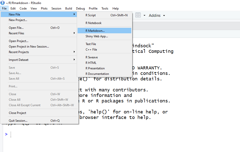
Start a new R markdown document in RStudio by clicking File > New File > R Markdown…
If this is the first time you have ever opened an R markdown file a dialog box will open up to tell you what packages need to be installed.
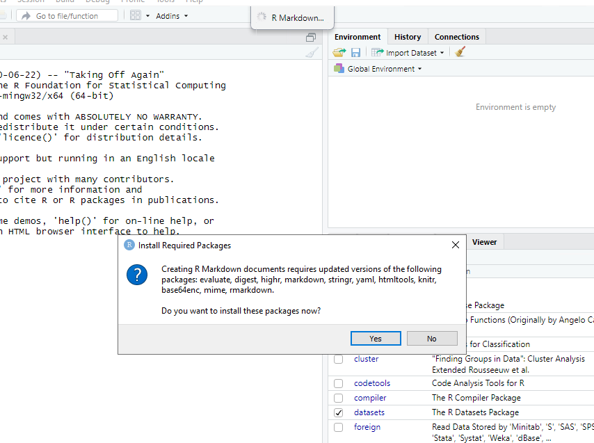
Click “Yes”. The packages will take a few seconds to install. You should see that each package was installed successfully in the dialog box.
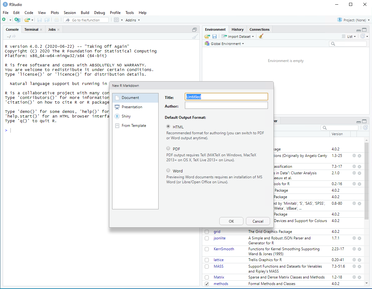
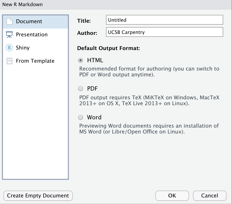
Once the package installs have completed, a dialog box will pop up and ask you to name the file and add an author name (may already know what your name is) The default output is HTML and as the wizard indicates, it is the best way to start and in your final version or later versions you have the option of changing to pdf or word document (among many other output formats! We’ll see this later).
New R Markdown will always pop up with a generic template…
If you see this template you’re good to go.
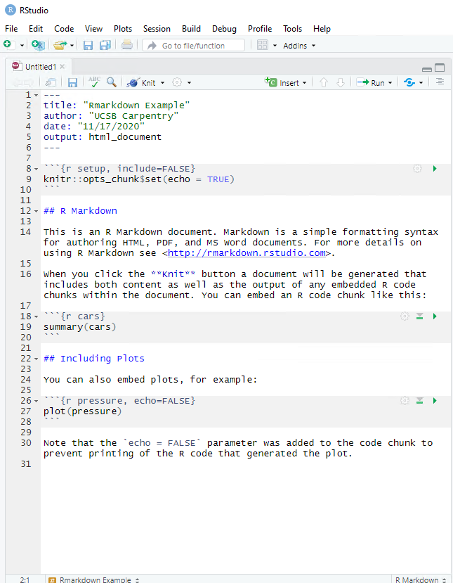
Now we’ll get into how our R Markdown file & workflow is organized and then on to editing and styling!
R Markdown Workflow
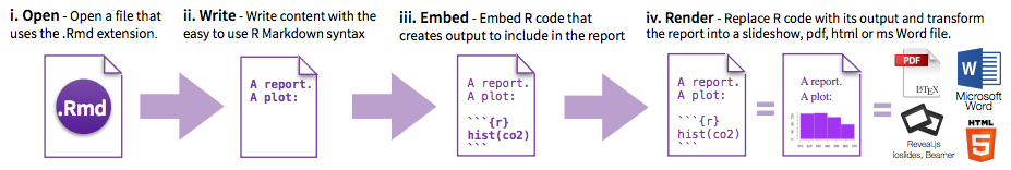
R Markdown has four distinct steps in the workflow:
- create a YAML header (optional)
- write R Markdown-formatted text
- add R code chunks for embedded analysis
- render the document with Knitr
Let’s dig in to those more:
1. YAML header:
What is YAML anyway?
YAML, pronounced “Yeah-mul” stands for “YAML Ain’t Markup Language”. YAML is a human-readable data-serialization language which, as its name suggests, is not a markup language. YAML has no executable commands though it is compatible with all programming languages and virtually any application that deals with storing or transmiting data. YAML itself is made up of bits of many languages including Perl, MIME, C, & HTML. YAML is also a superset of JSON. When used as a stand-alone file the file ending is .yml or .yaml.
R Markdown’s default YAML header includes the following metadata surrounded by three dashes ---:
- title
- author
- date
- output
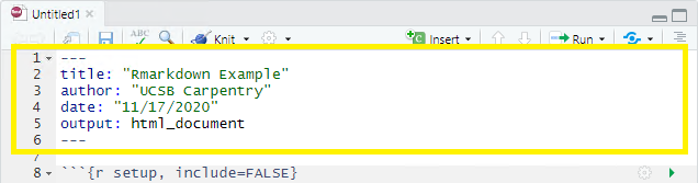
The first three are self-explanatory, but what’s the output? We saw this in the wizard for starting a new document, by default you are able to pick from pdf, html, and word document. Basically, this allows you to export your rmd file as a file type of your choice. There are other options for output and even more can be added by installing certain packages, but these are the three default options.
We’ll see other formatting options for YAML later on including how to add bibliography information, customize our output, and change the default settings of the knit function. Below is an example of how our YAML file will look at the end of this workshop.
---
title: "An Adapted Survey on Scientific Shared Resource Rigor and Reproducibility"
author: UCSB Carpentry
date: "December 16, 2020"
output:
  html_document:
    number_sections: true
bibliography: ../docs/bibliography.bibtex
csl: ../bin/apa-5th-edition.csl
knit: (function(inputFile, encoding) {
      out_dir <- '../results';
      rmarkdown::render(inputFile,
                        encoding=encoding,
                        output_file=file.path(dirname(inputFile), out_dir, 'Paper_Template_html.html')) })
---
2. Formatted text:
This one is simple, it’s literally just text narrative formatted by using markdown (more on markdown syntax later). Markdown-formatted text is one of the benefits added above and beyond the capabilities of a regular r script. Any text section will have the default white background in the rmd document. As you might know, in a regular R file, # starts a comment. In R markdown, plain text is just plain narrative text that appears in the document. In R scripts, plain text wants to be code. In R Markdown, you will need to enclose your code in special characters. Any symbols you do see that aren’t regular grammar components are for formatting, such as ##, ** **, and < >.
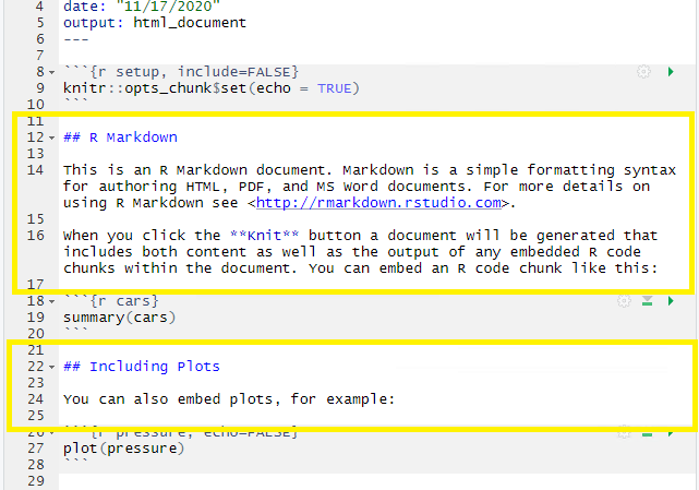
CHALLENGE 2.3 - Formatting with Symbols (optional)
In Rmd certain symbols are used to denote formatting that should happen to the text (after we “knit” or render). Before we knit, these symbols will show up seemingly “randomly” throughout the text and don’t contribute to the narrative in a logical way. In the generic Rmd document, there are three types of such symbols (##, **, <>) . Each symbol represents a different kind of formatting (think of your text formatting buttons you use in Word). Can you deduce from the surrounding text how these symbols format the surrounding text?
## R Markdown

This is an R Markdown document. Markdown is a simple formatting syntax for authoring HTML, PDF, and MS Word documents. For more details on using R Markdown see <http://rmarkdown.rstudio.com>.

When you click the **Knit** button a document will be generated that includes both content as well as the >output of any embedded R code chunks within the document. You can embed an R code chunk like this:
SOLUTION
##is a heading,**is to bold enclosed text, and<>is for hyperlinks. Don’t worry about this too much right now! This is an example of R Markdown syntax for styling, we’ll dive into this next.
3. Code Chunks:
R code chunks appear highlighted in gray throughout the rmd document. They are surrounded by three tick marks on either side (```) with the starting three tick marks followed by curly brackets {}with some other code inside. The tick marks indicate the start of a code section and the bits found between the curly brackets {}indicate how R should read and display the code (more on this in the Knitr syntax episodes). These are the sections you add R code such as summary statistics, analysis, tables and plots. If you’ve already written an R script you can copy and paste your code between the few lines of required formatting to embed & run whichever piece you want at that particular spot in the document.
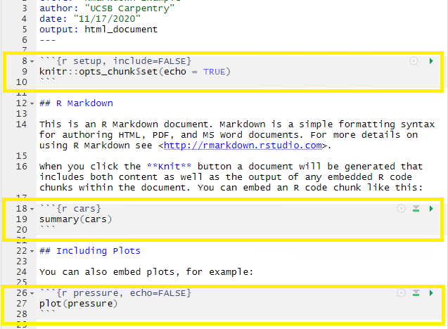
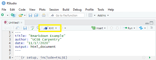
4. Rendering your Rmd document:
This is called “knitting”” and the button looks like a spool of yarn with a knitting needle. Clicking the knit button will compile the code, check for errors, and finally, output the type of file indicated in your yaml header. One nice thing about the knit button is that it saves the .Rmd document each time you run it. Your rmd document may not run and render as your indicated output if there are any errors in the document so it also functions somewhat as a code checker.
Try it yourself
We’re going to pause here and see what the R Markdown does when it’s rendered. We’ll just use the generic template, but when we’re working on our own project, knitting periodically while we’re editing allows us to catch errors early. We’ll continue rendering our rmd throughout the lesson to see what happens when we add our markdown and knitr syntax and to make sure we aren’t making any errors.
This is a little preview of what’s to come in the Knitr syntax episodes later on. Click the “knit” button
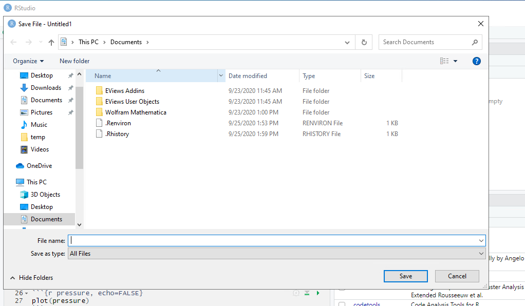
Before you can render your document, you’ll need to give it a file name and choose what folder you want to save it to. Choose rmd-workshop-paper.rmd as your file name and save the file to your code sub-folder.
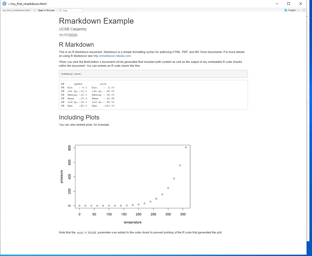
This is how our hmtl document will render after clicking the knit button and choosing a file name:
CHALLENGE 2.4 - echo=TRUE Function (optional)
Can you deduce what the echo=TRUE option stands for?
Solution
The echo=TRUE piece is knitr syntax that sets a global default for the whole paper. This piece of code specifically,
echo=TRUE, tells the rmd document to display the R code that generates the plots & analysis when the rmd document is rendered by hitting the “knit” button. Don’t worry too much about this now, we’ll learn more about this syntax in the Knitr Syntax episodes.
Starting our paper
Ok, now let’s start on our own rmd document.
Do this on your own in your new rmd file:
1) Delete EVERYTHING except the yaml header
2) Edit the yaml header to add the title of the paper we’re working on and to add yourself as author.
---
title: "An Adapted Survey on Scientific Shared Resource Rigor and Reproducibility"
author: [Add Your Name Here]
date: "December 16, 2020"
output: html_document
---
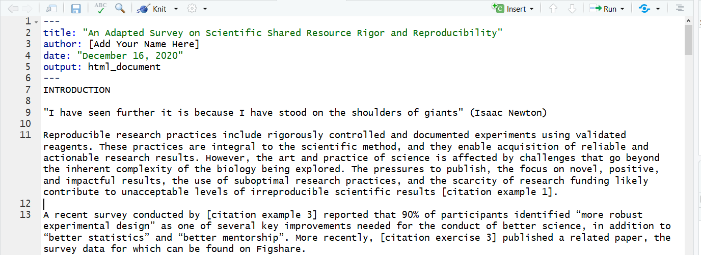
3) Navigate to the docs folder and open paper_raw.txt. Copy all the text with either ctrl-a or cmd-a then ctrl-c or cmd-c and paste ctrl-v or cmd-v AFTER the yaml header in our rmd file.
...
output:
  html_document
---
INTRODUCTION
Reproducible research practices include rigorously controlled and documented experiments using validated reagents. These practices are integral to the scientific method, and they enable acquisition of reliable and actionable research results. However, the art and practice of science is affected by challenges
...
Your file should now look something like this:
Now we’ll be set for our next episode which is about adding Markdown syntax to style your text sections (white sections)- including headers, bold, italics, citations, footnotes, links, citations etc.
Key Points
Starting a new Rmd File
Anatomy of an Rmd File (YAML header, Text, Code chunks)
How to knit an Rmd File to html
R Markdown Syntax: Headings & Lists
Overview
Teaching: 15 min
Exercises: 15 minQuestions
How does markdown in R compare to markdown in other programs?
How to create headings and sub-headings in R Markdown?
How to create bulleted and numbered lists in R Markdown?
Objectives
Understand how R markdown relates to the markdown universe
Learn how to create headings and sub-headings in R Markdown
Learn how to create bulleted and numbered lists in R Markdown
Intro to R Markdown Syntax
Before we dive into learning R Markdown Syntax, let’s talk a little about the “markdown” part.
R Markdown is a format for writing reproducible, dynamic reports with R which allows you to weave together narrative and code to produce elegantly formatted outputs. In practice, it allows you to use plain text for a document with bits of other things thrown in, but which will ultimately be converted to any number of other languages, for eventual display in the format you desire. It supports dozens of static and dynamic output formats such as HTML, PDF, MS Word.
The text in an R Markdown document is written with the markdown syntax, which is a basic markup language that conveys how text should be displayed. The basic markdown syntax has dozens of flavors, of which R Markdown is one. Most markdown syntax is preserved and works identically no matter what flavor you use. However, the different flavors will have different options or slightly different implementations of certain things.
R Markdown syntax is relatively simple and there are a number of tutorials and cheat sheets available online that you can consult while working on your reproducible report (here is a link explaining Pandoc’s markdown specs). In the next episodes we will be covering a subset of it, focusing on the most common formatting you may need to apply while writing reproducible documents.
First Things First - Line Breaks
It seems strange to have to talk about line breaks when writing text, but this is very important to know for proper rendering of your text. You will need to make sure to add line breaks into your document or text will wrap when it renders (even if you hit enter/return and start typing on a new line in R studio)
You can add line breaks by using :
- two spaces at the end of the line
- an html break
<br> - 2 enters/returns (leaving a blank line)
These line breaks will also be important to get your formatting to render correctly. In some cases you MUST have a blank line (just two spaces or a break won’t do the trick). Blank lines will be required before/after all headings, horizontal lines, and lists.
example:
If I'm writing some text
an enter should work for a line break, but doesn't

Here I am writing again,
I need to make certain I have a line break by:
adding two spaces
or an html break<br>
or by adding two returns

and I carry on writing
*Notice the spacing difference with 2 returns versus the other two options.
Creating Headings and Subheadings
Most papers or articles need headings and subheadings to distinguish different parts of the paper. We can insert headings and subheadings in R Markdown using the pound sign #. There are six heading/subheading sizes in R Markdown. The number of pound signs before your line of text determines the heading size, 1 being the largest heading and 6 being the smallest.
# Heading 1
## Heading 2
### Heading 3
#### Heading 4
##### Heading 5
###### Heading 6
Displays as:
Heading 1
Heading 2
Heading 3
Heading 4
Heading 5
Heading 6
Note this is Github’s markdown “flavor” for headers, they look different in R Markdown. However, relative sizing and hierarchy with 1 being the largest and 6 the smallest remains the same.
Tip: Add a Space!
It’s good practice to put a space between the last
#and the start of your heading. While R flavored markdown will still render#Title, other flavors of markdown (i.e. github) require a space between the#s and the heading text:# Title.
Numbered Sections
We would like to have numbered section headings in our paper. In order to do that we actually add a bit of code to the yaml section at the top.
Specifically, we will add a return to put html_document: on the next line indented (don’t forget to add the :), enter another line & indent again and then add number_sections: true.
It should look like the following:
```
---
title: "An Adapted Survey on Scientific Shared Resource Rigor and Reproducibility"
author: Add Your Name Here
date: "December 15, 2020"
output:
  html_document:
    number_sections: true
---
```
We want to insert headings and subheadings to divide our paper into more readable parts. Let’s start by adding one at the beginning to start our introduction.
To conform to markup best practices, header 1 # should only be used for the title. From there, for each sub-heading level you use one heading level lower, for example the introduction will be header 2 ##.
Tip: More Heading Convention
For best practices regarding all heading levels, you should never skip a heading level - heading levels inform the hierarchy of your paper compositions, they do not reflect styling choices. For styling you may employ CSS stylesheets, either importing an exisiting “theme”, or creating your own.
In the first line of our paper, make the word “Introduction” into a heading 2 by adding a ## before the line.
## INTRODUCTION
Now let’s knit to see how the heading is formatted.
Oops! for our Introduction we have 0.1 Introduction. The numbering isn’t right here…
What’s going on?
This is an exception in R Markdown. Because an R Markdown document defines the title within the YAML header, you should actually use header 1 # for the next highest header level after the title, (Introduction, Conclusion, etc.). Otherwise, if you use numbered sections, the numbering will be off.
So, let’s try this again, this time with heading 1 #:
# INTRODUCTION
Now we can go to the next section and add a main heading and a subheading. Find the “Materials and Methods” section (right after the introduction) and make the line that says “Materials and Methods” into heading 1 and the lines that say “Survey Overview” and “Data Analysis” into heading 2 for subheadings.
# MATERIALS AND METHODS
## Survey Overview
## Data Analysis
Tip: Finding Content on RStudio
Use Ctrl+F (Windows) or Command+F (Mac) shortcut keys, or from the Edit -> Find to locate content in your paper. We will be using that quite a lot during this workshop.
CHALLENGE 3.1 - Applying Headings and Subheadings
Insert headings and subheadings throughout the rest of the paper.
Make these lines into headings so our paper is split into 5 main sections:
- Introduction (already done)
- Materials and Methods (already done)
- Results and Discussion
- Conclusion
- References
Make these lines into subheadings:
- Survey Overview (already done)
- Data Analysis (already done)
- Survey Demographics
- Current Landscape for Rigor and Transparency in Represented Shared Resources
- Core Implementation of Research Best Practices
- Strategies for Improving R&R in Core Operation
Think carefully about which heading levels you should use for consistency throughout your paper. *Use the search function in R Markdown
ctrl-forcmd-fto find these lines in the document quickly.SOLUTION
# INTRODUCTION
# MATERIALS AND METHODS
# RESULTS AND DISCUSSION
# CONCLUSION
# REFERENCES

## Survey Demographics
## Current Landscape for Rigor and Transparency in Represented Shared Resources
## Core Implementation of Research Best Practices
## Strategies for Improving R&R in Core Operation
## Creating Bulleted and Numbered Lists
Time to Knit!
Check how the headings look like in your paper.
Horizontal Lines
If you wish to create divisions between sections, you can insert a horizontal line in using 3 (or more) dashes, asterix, or underlines (---, ***, or ___):
---

See some paragraph text
between horizontal lines---
Now you know markdown

***
The above renders as:
See some paragraph text
between horizontal lines—
Now you know markdown
*Note again that displayed here is the github styling for horizontal lines, they look different rendered in R Markdown
Tip: Leave Blank Line Before & After Horizontal Lines
Depending on the platform, the markdown parser may interpret your attempt at a horizontal line as some other styling unless you add a blank line before and after the line. A break
<br>may not even work, it should be a completely blank line.
Ok, let’s add a horizontal line in our paper under the title:
--- (yaml end)

---

# INTRODUCTION
Time to Knit!
Check how the horizontal line looks in your paper
CHALLENGE 3.2 - Adding Horizontal Lines (optional)
Add horizontal lines after each section header.
SOLUTION
# INTRODUCTION

***

# MATERIALS AND METHODS

***

# RESULTS AND DISCUSSION

***

# CONCLUSION

***

# REFERENCES

***
Bulleted & Numbered Lists
Academic articles often include lists to make important findings stand out more or to summarize key points for readers. We will learn how to create both unordered lists with bullet points, and ordered numbered lists.
Unordered Bullet Lists
Creating unordered lists is relatively simple. For unordered lists, you can use: asterix, dash or plus characters *, - or +:
* A bullet point
- Also a bullet point
+ Still a bullet point
Outputs as:
- A bullet point
- Also a bullet point
- Still a bullet point
You can also add sub-levels, to create sub-lists by indenting the next list item evenly by two or four spaces:
* A bullet point
  * Sub-level one
    * Sub-level two
Outputs to:
- A bullet-point
- Sub-level one
- Sub-level two
- Sub-level one
Ordered Numbered Lists
For ordered lists, you use a number with a dot, e.g: 1. Your numbers do not need to be sequential. Markdown will number the item in the order in which they appear rather than their numeric order.
1. First item in our numbered list
7. Second item in our numbered list
2. Third item in our numbered list
The above will appear as:
- First item in our numbered list
- Second item in our numbered list
- Third item in our numbered list
Tip: No ) for Numbered Lists
Markdown parser does not accept parenthesis as a list delimiter, so if you use parenthesis, the output will be the same as above. i.e.
1)outputs as1..
CHALLENGE 3.3 - Inserting Bullet Points
Now let’s practice creating bullet lists. Search in the paper “it is important to highlight:” and apply bullet points for each of the next 3 sentences.
SOLUTION
* At least 170 (∼80%) respondents use documentation, in the form of quality control and standard operation procedures (SOPs) to support practices.
* The incorporation of an instrumentation management plan, was not as highly utilized (56%).
* Oversight of data analyses and double-checking results were some of the least widely used ones (26%).
Remember: You can use
+or-too.
CHALLENGE 3.4 - Applying Numbered Lists
Use RStudio to locate the paragraph which ends with “in grant applications, as follows:” the next four sentences should be shown as numbered a list.
SOLUTION
1. scientific premise forming the basis of the proposed research
2. rigorous experimental design for robust and unbiased results
3. consideration of sex and other relevant biologic variables
4. authentication of key biologic and chemical resources
Time to Knit!
Check how the bulleted & numbered lists looks like in your paper.
If needed, you can also combine sub-levels numbers or even combine bullets and numbered items in the same list, by indenting different levels.
Key Points
Heading syntax (#,
Bulleted lists (*, - , or +)
Numbered lists (1., 2., etc.)
R Markdown Syntax: Hyperlinks, Images & Tables
Overview
Teaching: 10 min
Exercises: 10 minQuestions
How do I create hyperlinks in R Markdown?
How do I insert images or tables into R Markdown?
How do I resize images?
Objectives
Learn how to add hyperlinks to an R Markdown document
Find out how to insert images into an R Markdown document
Learn how to add tables into an R Markdown document
Creating Hyperlinks
Hyperlinks are created using the syntax [text](link) with no spaces in between the parentheses and the square brackets.
For example:
[RStudio](https://www.rstudio.com)
Now, let’s apply it to the template paper. Find where the “Center of Open Science” is mentioned and link the institution to their official website:
[Center for Open Science](https://www.cos.io/)
Time to Knit!
Check if you hyperlinks are working properly.
Challenge 4.1: Adding links
Let’s add another link to our paper. Now it is your turn! We want to create a hyperlink to the survey platform used in the study Survey Monkey (https://www.surveymonkey.com/).
Solution
[SurveyMonkey](https://surveymonkey.com)
Tip:
You can use html directly in your .rmd document to add a link that will open in a new tab, such as
<a href="http://www.ucsb.edu/" >target="_blank"> UCSB</a>. This syntax requires pandoc and link_attributes extension, that is by default included in R Markdown.
Inserting Images
You can add images to an R Markdown report using markdown syntax as follows:

You’ll notice this format is exactly the same as hyperlinks, but with the addition of an ! before the brackets and parentheses.
However, when you knit the report, RStudio will only be able to find your image if you have placed it in the right place - RELATIVE to your .Rmd file. This is where good file management becomes extremely important. We have placed all our images in the figs folder in the R-markdown project folder. In that case, make sure your path starts with ../figs/ along with the correct image name and file extension. Also the closing bracket and the opening parentheses should be close to each other, without any spaces in between.
Tip: Paths to Files
The specification of the list of folders to travel and the file name is called a path. A path that starts at the root folder of the computer is called an absolute path. A relative path starts at a given folder and provides the folders and file starting from that folder. Using relative paths will make a number of things easier. A path is made up of folder names. If the path is to a file, then the path will ends with a file name. The folders and files of a path are separated by a directory separator. There are a few special directory names. A single period
.indicates the current working directory. Two periods..indicates moving up a directory.
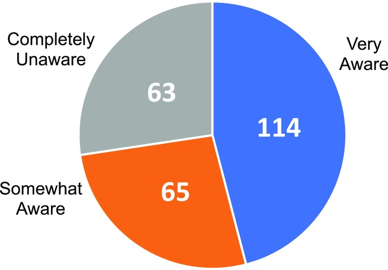
In our paper template there are three images (two pie charts) and one bar chart we want to include. Those are named fig1_paper.jpg, fig2_paper.jpg and fig3_paper.jpg.
To start let’s identify where Fig. 1 is mentioned in the paper. We will insert the image right after that. This image will have the caption labeled “FIGURE 1 - Knowledge and awareness of the current NIH guidelines on rigor and reproducibility.” (that we will be pasting in the chat). We need that caption to render the image.
The markdown should look like:

Note: A preview of your image should pop up automatically in RStudio if you have the correct relative path. But this will be only true if you type out the code, not if you copy and paste it.
This will output as:
Resizing Images
The image you just added looks a little too big, right? We can resize it by adjusting the width and height ratio. Let’s say we want this image to be half of the original size. In order to do that, we will have to add to the syntax:
{width=50% height=50%}
This will output as:
CHALLENGE 4.2 - Inserting Images
Locate the places for Fig. 2 and Fig. 3 and add them to the document using the captions below:
FIGURE 2 - Lack of requests for rigor and reproducibility documentation by users of shared resources
FIGURE 3 - Types of tools that cores would like to implement in their operations
*The bar chart should use a ratio of 60% x 80% in order to improve readability.
Solution:
{width=50% height=50%}{width=60% height=80%}
Time to Knit!
Check how your images look now.
Inserting Tables
We can also use markdown syntax to insert a formatted table into our document. The basic syntax to insert a table looks like this:
Column Header | Column Header
---           | ---
Cell 1        |  Cell 2
Cell 3        |  Cell 4
Output:
Column Header | Column Header
— | —
Cell 1 | Cell 2
Cell 3 | Cell 4
Start with the column names/headers. Separate columns with the pipe ( | ) symbol. Right below the column headers use at least three dashes to separate the headers from the cells of the table. Then fill in the contents of the table row by row, separating columns using the pipe ( | ) symbol.
Note: Table Spacing
the spacing between cells in each row can help with readability in the R Markdown file, but is not necessary to get the correct output. As long as the pipe symbol is there, R Markdown will automatically format the table in your output. The following syntax will print the same table as the spaced out table above.
Column Header|Column Header
--- |---
Cell 1|Cell 2
Cell 3|Cell 4
You can use text emphasis in the table using the same syntax as you use when emphasizing other plain text. The following change will bold the column headers in the output.
 **Column Header** | **Column Header**
 ---               | ---
 Cell 1            |  Cell 2
 Cell 3            |  Cell 4
Output:
| Column Header | Column Header |
|---|---|
| Cell 1 | Cell 2 |
| Cell 3 | Cell 4 |
Let’s create Table 1 in our paper in section 3.2 Current Landscape for Rigor and Transparency in Represented Shared Resources.
Start with the column headers “Category” and “N” in bold. Then add the separator between the header and the cells. We’ll also type out the first two rows of the table.
**Category** | **N**
--- | ---
Poor sample quality from users/sample variability/limited biological material | 51
Lack of well-trained principle investigators and lab members/Poor oversight | 45
CHALLENGE 4.3 - Complete the Table
Finish Table 1 by adding the rest of the rows.
SOLUTION
**Category** | **N**
--- | ---
Poor sample quality from users/sample variability/limited biological material | 51
Lack of well-trained principle investigators and lab members/Poor oversight | 45
Poor experimental design: Lack of sufficient replicates/inadequate sample size/lack of adequate controls | 43
Inadequate standardization of protocols or guidelines, and data analysis | 43
Cost and time | 39
Failure to leverage the core’s expertise/following the core’s advice/no consulting beforehand | 23
Inadequate documentation of experiments/data management | 19
Instruments: maintenance, upgrades, changes | 15
Responses that could not be assigned to a category | 11
Time to Knit!
Check how the table you have just created looks like.
Note: Advanced & Interactive Tables
There are some packages that allow you to make more advanced and interactive tables. Here are some references for these packages: https://cran.r-project.org/web/packages/kableExtra/vignettes/awesome_table_in_html.html and https://www.htmlwidgets.org/showcase_datatables.html
Key Points
R Markdown syntax for hyperlinks
R Markdown syntax for images
You can resize images with R Markdown
You can easily create basic tables with R Markdown
R Markdown Syntax: Emphasis, Formulas & Footnotes
Overview
Teaching: 10 min
Exercises: 10 minQuestions
How do I emphasize text in an R Markdown document?
How do I add LaTex formulas?
How can I make superscript text?
How can we add footnotes?
Objectives
Learn how to apply emphases to words or phrases in R Markdown
Understand the power of LaTeX (Lay-techhh) for mathematics formatting
Learn how to add equations and formulas in R Markdown
Learn how to add footnotes in R Markdown
Adding Emphasis
Another way we can customize our R Markdown file output is by emphasizing words or phrases. In our paper, there are several instances of words and phrases that are italicized or bolded. We use markdown syntax to add these emphasis to words or phrases by surrounding them with matching symbols. Different symbols give different emphases effects.
Put text in italics with single asterisks or single underscores.
*italics* will give output italics
_italics_ will give output italics
Make text bold with double asterisks or double underscores.
**bold** will give output bold
__bold__ will give output bold
Let’s try that italics applying that to two organization names that appear in the text. First let’s put the Association of Biomolecular Resource Facilities in italic. _Association of Biomolecular Resource Facilities_ or *Association of Biomolecular Resource Facilities* will render Association of Biomolecular Resource Facilities. Now try the same with the Committee on Core Rigor and Reproducibility.
CHALLENGE 5.1 - Applying Bold Emphasis
For testing out making the text bold, let’s search for the mention to the Transparency and Openness Promotion in the paper and make them bold.
SOLUTION
Either
__Transparency and Openness Promotion__or**Transparency and Openness Promotion**will render Transparency and Openness Promotion
Which symbol do you prefer to use? Do you prefer to stick with the same for both emphases?
Time to Knit!
Check how the emphases you have just applied looks like in your paper.
Tip: When you realllllly want to emphasize something
you can combine emphasis styles by combining the symbols surrounding the word or phrase. Make text bold and italicized with triple asterisks or triple underscores.
***super emphasized***will give output super emphasized___super emphasized___will give output super emphasized
Adding Blockquotes
R Markdown also allows you to emphasize a pull quote using blockquotes. Let’s say you want to transform the first sentence in the paper into one and also apply italic emphasis. For this you will have to add a carrot “>” (greater-than symbol) and the asterisc or underscore for the italics, as demonstrated below:.
>_"I have seen further it is because I have stood on the shoulders of giants"_ (Isaac Newton)
The output you will get shoul look like that:
“I have seen further it is because I have stood on the shoulders of giants” (Isaac Newton)
Time to Knit!
Check for the block quote in your paper.
Adding Equations & Formulas
LaTeX (pronounced Lay-techhh) is a comprehensive document formatting and preparation system. It is very powerful, but also famously difficult to use. A few journals require that papers be written in LaTeX, and some fields, such as high energy physics, use it exclusively. Why? Because, despite its difficulty, its mathematics formatting (its formatting of equations and formulas) is better than anything else out there.
RStudio has a most wonderful feature that allows you to use just the mathematics formatting portion of LaTeX without having to use LaTeX as a whole, without having a LaTeX installation on your system, and without having to understand LaTeX generally.
An inline formula is delimited with single dollar signs, as in $ 2+2 = 4 $. A display equation uses double dollar signs, $$ 2+2 = 4 $$. What goes between the single or double dollar signs is LaTeX math formatting. This is its own language, and you just have to learn it. A decent online reference (Overleaf is an online LaTeX editor):
The canonical LaTeX reference, written by the author (hardback, but viewable online):
- https://archive.org/details/latex00lesl
- https://ucsb-primo.hosted.exlibrisgroup.com/permalink/f/1egv95m/01UCSB_ALMA21230090630003776
But, know that the LaTeX math language is very intuitive once you get a feel for its style. Put your math head on, not your programming head. If you want to say that a equals b times c, in a programming language you might write something like a = b*c, but in LaTeX you would say $ a = bc $. Spaces generally don’t matter in LaTeX; it “understands” your formula and uses rules to determine how to display things.
Challenge 5.2 - Adding Formulas
Let’s add the following text and formula to our data analysis section where the paper talks about confidence level:
Using the sampling error formula
$$e = { Zp(1-p) \over \sqrt{n} }$$we compute that at a 95% confidence level (i.e., Z=1.96), with base probability p=1/2 and sample size n=243, the margin of error is +/-3%.
Time to Knit!
Check how the formula just rendered in your paper.
Double click on the equation. Notice how RStudio gives you a preview of it. Nice! The formula here uses curly braces for grouping (kind of like invisible parentheses). \over gives a fraction with a big horizontal line. Try replacing that with just / for an alternative rendering.
Challenge 5.3 - Inline Formulas
For inline formulas, in the same section of text replace
Z=1.96with$Z=1.96$and similarly. Notice the different formatting, and notice again RStudio’s preview when you hover over the formula. In LaTeX, you would say$ \pm 3 \% $for the +/-3%. Later we’ll see how to have R compute this value inline.
Time to Knit!
Check how the new formulas just rendered in your paper.
To appreciate the beauty of LaTeX’s typesetting, just look at how formulas are typeset by other systems. Here’s an example: https://www.educba.com/confidence-interval-formula/
RStudio’s facility to bring in LaTeX for math formatting makes it a wonderful authoring environment for math-rich papers that are not computational and have nothing to do with R at all.
Adding Footnotes
We can add footnotes to our paper using the ^. Similar to adding emphasis, putting carrot symbols around your text will print the output as a superscript.
^superscript^ will give output: superscript
footnote^1^ will give output: footnote1
In our paper, we will create a footnote in the introduction when we reference a notice from the U.S. National Institutes of Health (NIH). We will add a footnote after the word “notice” by adding ^1^ right after the word.
notice^1^
Challenge 5.4: Creating Footnotes
Let’s add a footnote to our paper. Right before the References section, add a superscript to distinguish the footnote and match it with the inline footnote. The text to the footnote will be: Through these four elements, the NIH intends to “enhance the reproducibility of research findings through increased scientific rigor and transparency” https://ori.hhs.gov/images/ddblock/ORI%20Data%20Graphs%202006-2015.pdf`
Solution
^1^Through these four elements, the NIH intends to...
Time to Knit!
Take a look at the footnote you have just created.
Key Points
You can add *italicized* and *bolded* texts in R Markdown
There is an extensive LaTeX guideline for mathematics formatting
You can add create superscript text & linked footnotes
R Markdown Syntax: Citations & Bibliography
Overview
Teaching: 20 min
Exercises: 10 minQuestions
How to include citations?
How to create a list of references?
How to apply different citation styles?
Objectives
Learn how to include citations
Create a list of references
Learn how to apply different citation styles
Getting the Bibliography
Let’s now move our attention to include citations and list out the references (bibliography) in our paper example. Before adding citations we need to list out all citable items and set a bibliography. In order to add a bibliography we will need to include a bibliography file in the YAML header. Bibliography formats should be specified in one of the formats supported by Pandoc on RStudio:
- MOD: .mods
- BibLaTeX: .bib
- BibTeX: .bibtex
- RIS: .ris
- EndNote: .enl
- EndNote XML: .xml
- ISI: .wos
- MEDLINE: .medline
- Copac: .copac
- JSON citeproc: .json
Note that bibliography formats are not the same as citation styles. These are specified by a CSL (Citation Style Language) that we will cover later on. For now, we will stick to the bibtex format supported by Google Scholar, which will be used to retrieve example references for our practice paper. If you use a reference manager such as Zotero, Endnote, Mendeley etc. to manage your library, you can also export the .bibtex file directly, with all citable items you consider to include in the paper.
A *.bibtex file consists of bibliography in plain-text format. Go to your R-markdown project folder, then paperToRmd then docs and open the bibliography.bibtex. We already have a couple of citable items listed in this file. Let’s take a closer look to understand their anatomy:
@misc{nature_nature_2018,
	type = {Repository},
	title = {Nature {Reproducibility} survey 2017},
	url = {10.6084/m9.figshare.6139937.v4},
	journal = {Figshare},
	author = {Nature},
	year = {2018},
}

@article{springer_reality_2016,
	title = {Reality check on reproducibility.},
	volume = {533},
	doi = {10.1038/533437a},
	number = {7604},
	journal = {Nature},
	author = {Springer, Nature},
	month = may,
	year = {2016},
	pages = {437},
}
Note that the first line specifies the type of citation, MISC for miscellaneous, and Article for papers, along with the main entry which will be used to link in-text citations further in the episode. The other lines include the metadata that describes different parts of the bibliography, such as the date, the author, etc.
Let’s now understand the process of how to get a bibtex, using as example the item 1,500 scientists lift the lid on reproducibility authored by Baker (2016), following the steps below:
- 1) Search for the first paper listed on Google Scholar by copying and pasting the title of the paper. Make sure to use quotations to better filter results and get the right paper. A tricky part is that if you want more complete files that will render to more accurate citations you have to check for all existing versions of the same result (if any). Google Scholar amasses them altogether into one in the link “All 6 versions”, listing out different repositories and websites the paper can be found.
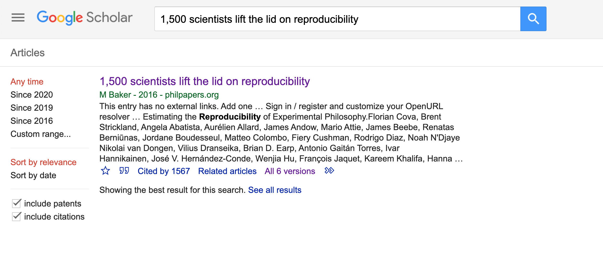
- 2) Click on the link to check for other existing versions. The first result does not include the journal name, so let’s choose the second one instead, which won’t require us to adjust the metadata.
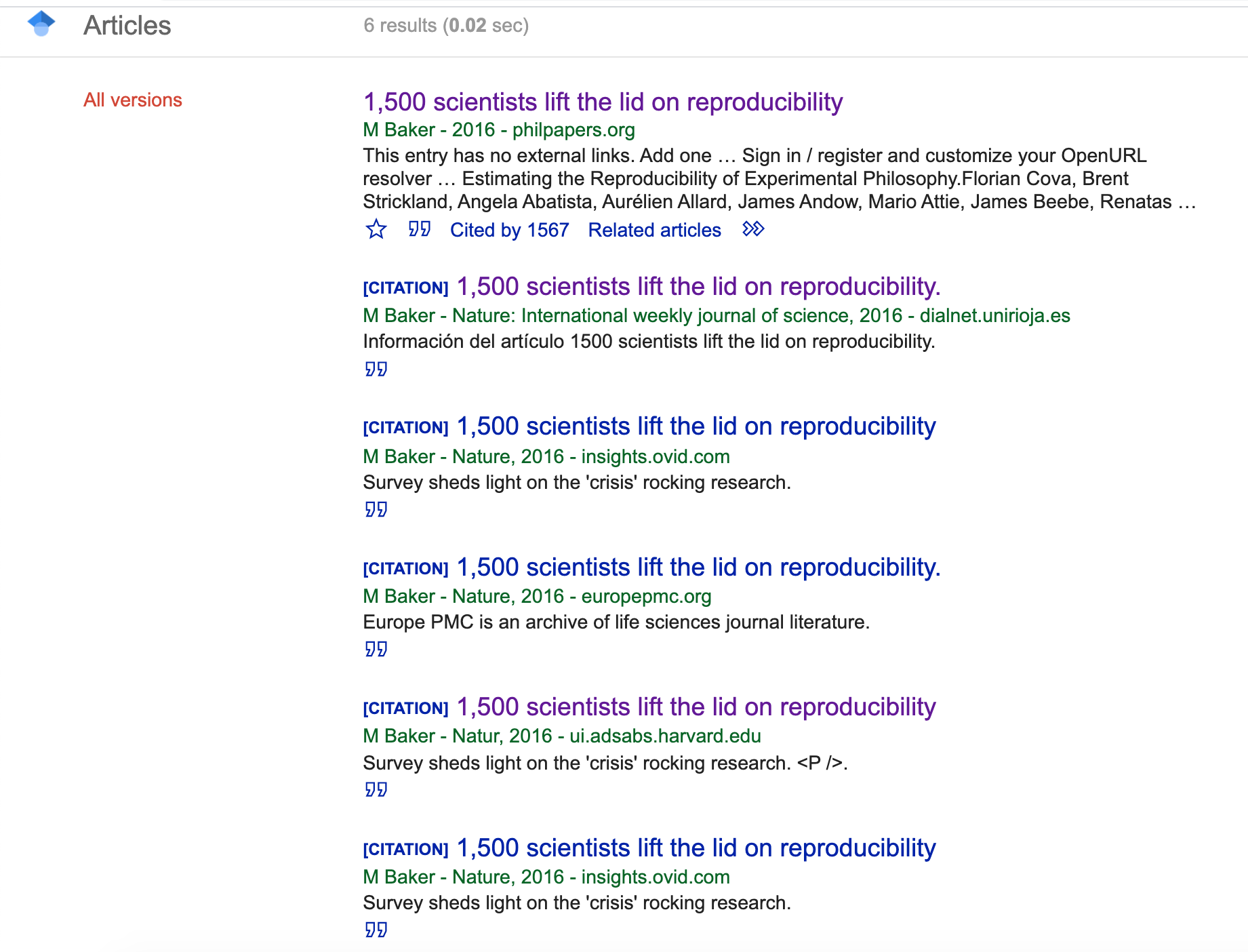
- 3) When you click on the quotation icon right below the version you chose, it will prompt a window that will give you the option to choose BibTeX.
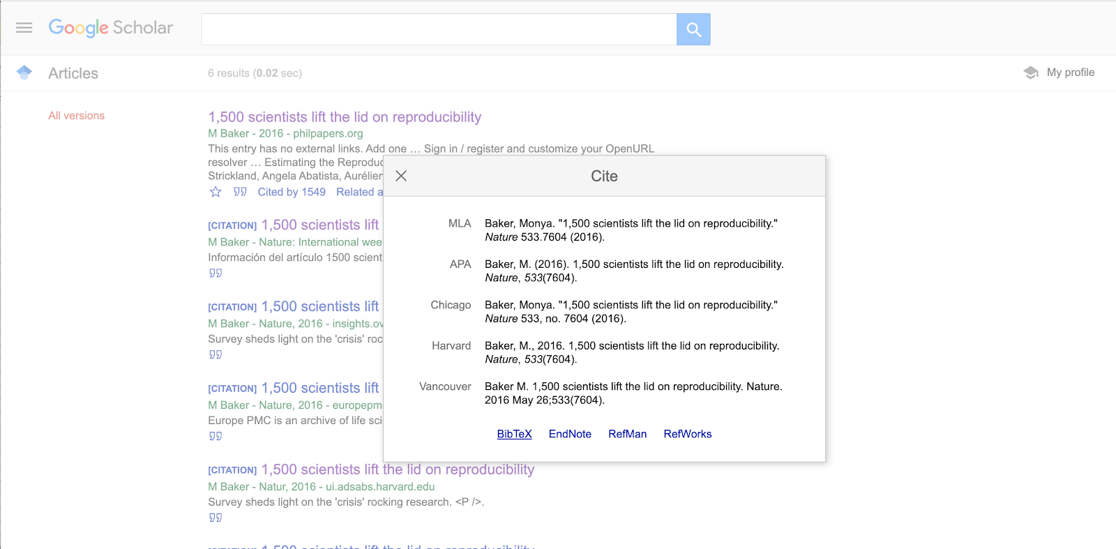
- 4) Choose the BibTeX option. It will prompt a file in your browser, like this:
@article{baker_1500_2016,
	title = {1,500 scientists lift the lid on reproducibility},
	volume = {533},
	url = {http://www.nature.com/news/1-500-scientists-lift-the-lid-on-reproducibility-1.19970},
	doi = {10.1038/533452a},
	abstract = {Survey sheds light on the ‘crisis’ rocking research.},
	language = {en},
	number = {7604},
	urldate = {2020-11-13},
	journal = {Nature News},
	author = {Baker, M.},
	month = may,
	year = {2016},
	pages = {452},
}
- 5) If you did not have that item already you would simply copy and paste this to your bibliography.bibtex file. The order would not matter, since references will be listed according to the style. It is strongly recommended to have entries separated by blank lines though. That makes them look like paragraphs, and easier to locate.
Tip: How can you get many bibtex at once?
Alternatively, you can also conduct multiple searchers and save results to your personal library on Google Scholar and export multiple items as .bibtex files in a bulk.
We already have .bibtex file with all items we need to proceed. But how will RStudio be able to link this file with the .rmd file on the other tab? Well, remember we mentioned before that we should include a bibliography file in the YAML header? In this case we will add to the existing YAML the following information:
---
bibliography: "../docs/bibliography.bibtex"
---
Note again the importance of the relative path calling the right folder. The connection between the two files is all set to get us started. For now, we won’t need to specify which format we would like to use.
By default, Pandoc will use a Chicago author-date format for citations and references and we will stick with that for now, but later we will learn how to change citation styles.
Adding Citations
Each item in the bibliography.bibtex file starts with a @ entry which specifies the type of document followed by a curly opening bracket which specifies the key that should be included to create in-text citations.
We will call a citation using the @ followed by the key. It is important to use this exact key in the .bibtex to render correct mentions in the text. Let’s see how that should be included in the R Markdown syntax for different types of citations.
Single citation
At the end of the first paragraph on the Introduction, where you find [citation example 1]. Remove this info and let’s practice adding our first citation. Let’s use the item with the key freedman_2020_2017 from the bibliography.bibtex file in the second tab. In order to cite this work you should add this key after in between brackets, as follows:
[@freedman_2020_2017]

The output you will get in Chicago style will be:

(Freedman, Venugopalan and Wisman 2017)
Challenge 7.1: Adding single citation
Locate
[citation exercise 1]in the document, and replace it by a citation to Munafo’s (2017) study.Solution
[@munafo_manifesto_2017]The output you will get in Chicago style will be:(Munafo, 2017)
Multiple Citations
If you want to add multiple citations in a row (same parentheses) you will have to separate keys by semicolon. So let’s add Bustin (2014) and Freedman, Venugopalan and Wisman (2017) to [citation example 2]
[@bustin_reproducibility_2014; @freedman_2020_2017]
The output you will get in Chicago style will be:
(Bustin, 2014; Freedman, Venugopalan and Wisman, 2017)
Tip: You can simplify items key if you want. For instance, you can keep only the first author and year, but for the purpose of the exercises we will keep keys exactly how we got them from Google Scholar.
Challenge 7.2: Adding multiple citations
Now it is your turn! Locate in the document the note
[citation exercise 2]. Remove it and include a citation to Baker (2016) and Freedman, Venugopalan and Wisman’s (2017) studies.Solution
[@baker_1500_2016; @freedman_2020_2017]The output you will get in Chicago style will be:(Barker, 2016; Freedman, Venugopalan and Wisman, 2017)
Keeping Authors in the narrative
There are cases authors are announced in the text, and therefore their names shouldn’t go between parentheses. Let’s say you want to add a citation to support the statement about Springer’s survey. In order to keep the institutional author out of the parentheses, we should add a hifen - before the @ followed by the citation key. Let’s add that to the [citation example 3] remark on the paper.
In that case you’ll have to first type in the last name(s) of the author(s) as only the year will be rendered. For this example the author is an organization, so let’s type Springer, then enter the key for the item, as follows:
“A recent survey conducted by Springer [-@springer_reality_2016] reported that 90%…”
The output you will get will be:
“A recent survey conducted by Springer (2016) reported that 90%…”
Challenge 7.3: Keep author(s) in the narrative
Let’s practice now how to insert citations outside the parantheses! In the same paragraph, where you find
[citation exercise 3]add a citation (year only) to your mention to Nature’s survey in order to indicate the dataset you are referring to.Solution
[-@nature_nature_2018]Did you remember to type in the organization who authored the publication? If so, the output you will get should be:Nature (2018)
Time to Knit!
Check how the citations you have just created renders in your paper.
Setting the Reference List
All cited items will be listed under the section References which you created before while practicing headings and subheadings. Items will be placed automatically in alphabetical order.
Adding an item to a bibliography without citing it
By default, the bibliography will only display items that are directly referenced in the document. If you want to include items in the bibliography without actually citing them in the body text, you can define a dummy nocite metadata field in the YAML and put the citations there.
nocite: |
  @item1, @item2
To demonstrate that I will add a new bibtex from my Google Scholar Library and specify the @keyin the YAML. Note that this will force all items added in the YAML to be displayed in the bibliography.
Changing Citation Styles
There are a number of existing citation styles (CSL), but we won’t cover their differences and applications during this workshop. To use another style, we will need to specify a CSL (Citation Style Language) file in the metadata field in the YAML header.
Let’s assume that we want to use the APA 5th edition apa-5th-edition.csl instead. In order to do so, you have to make sure the CSL you want to apply is correctly named in the YAML, matching the .csl file saved in the project folder and opened in RStudio. We have done that for you. The csl for APA is saved in the bin folder, so using the relative path to the file, we will include that to the YAML:
csl: ../bin/apa-5th-edition.csl
Time to Knit!
Knit the document and note that citations and references now conform to the APA style.
Tip: Change the CSL default
You can override this default by copying a CSL style of your choice to default.csl in your user data directory.The CSL project provides further information on finding and editing styles. More information about CSL can be found here https://docs.citationstyles.org/en/1.0.1/primer.html.
Key Points
R Markdown supports different citation styles
Finding & Applying Existing Journal Templates
Overview
Teaching: 10 min
Exercises: 0 minQuestions
What is the advantage of using the rtciles package?
How to find existing journal templates?
Objectives
Learn about the rticles package and its functions
Locate existing templates for creating R Markdown papers and reports
Installing the “rticles” Package
We have learned how to start a new document on RStudio and apply some important R Markdown syntax to format your reports. But, let’s say you are writing a paper and you already know which journal you are submitting it to. Writing it in your own style and then formatting prior to submission would be too time-consuming, right? The good news is that RStudio can make our lives easier! Through a package called “rticles” you can access a number of existing journals’ templates that will let you easily and quickly format and prepare your paper draft for peer review.
Let’s take a look at that! On RStudio, install the package using the command install.packages("rticles") or by clicking install on the right-hand side pane and typing rticles. Once the installation is completed, use the plus icon at the upper-left side of your screen to create a new document or proceed with File>New File>Markdown. This will prompt the window bellow:
Clicking on “from template” will prompt a couple of dozen templates listed as {rticles}. Let’s choose the Biometrics Journal template and then, OK.
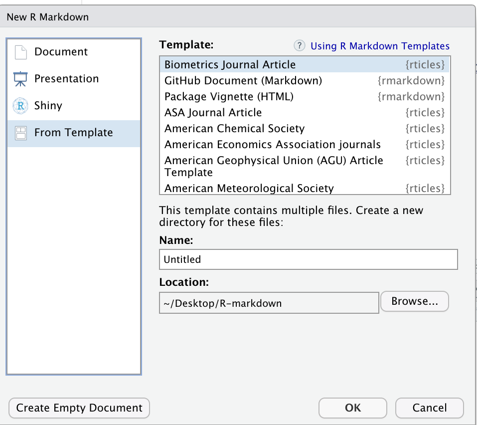
Note that along with the skeleton of the paper you will see a message on top indicating additional packages you may need to install for that particular template. Creating templates and adding other templates is beyond the scope of this workshop, but that is also possible. To learn more you can check the link Using R Markdown Templates on the right-hand side or check the rticles package documentation.
Key Points
The rticles pachage provides some journal templates
Whenever available, if you already know which journal you are submitting to, start your paper using the template
Knitr Syntax: Inline Code & Code Chunks
Overview
Teaching: 40 min
Exercises: 15 minQuestions
What is “Knitr”?
When would I want to add inline code?
How to add inline code?
When would I want to use code chunks?
How do I add code chunks?
Objectives
Understand the basic functions of Knitr
Learn how to add inline code to your document
Learn how to add code chunks to your document
Distinguish when inline code vs. code chunks would be appropriate
Understand how to change the output characteristics of code chunks
What is Knitr?
Knitr is the engine in RStudio which creates the “dynamic” part of R markdown reports. It’s specifically a package that allows the integration of R code into the html, word, pdf, or LaTex document you have specified as your output for r markdown. It utilizes Literate Programming to make research more reproducible. There are two main ways to process code with Knitr in R Markdown documents:
- Inline code
- Code Chunks
Adding Inline code
Inline code is best for calculating simple expressions integrated into your narrative. For example, use inline code to calculate an error margin or summary statistic, such as # of observations, of your dataframe in your results section. One of the benefits of using this method is if something about your data set changes (like leaving out NAs or null values) the code will automatically update the calcuation specified.
We’re going to go ahead and change the LaTex code we used to input the error margin and calculate it dynamically using r code. So, instead of $ \pm 3 \% $ to display our error margin as +/-3%, let’s add this:
`r round(1.96*0.5*(1-0.5)/sqrt(243)*100)`%
Notice how we put the % sign after the ticks. In this case the percentage sign should be plain text. If we had put it inside the ending backtick (`) r would have attempted to calculate the modulo since that’s what that symbol stands for in R.
Time to Knit!
See that inline code evaluates to calculate the error margin of +/- 3%.
Where else can we add inline code? We can replace observation counts!
i.e. “There are #r nrow(my_data) individuals who completed the survey”
Now, we’re going to find one such example in our data frame and convert a static number or equation to inline code. In our paper text we read “a total of 243 individuals from 21 countries completed this section.” Here we can use inline r code to calculate the total responses instead of typing it in.
However, because we don’t have access to the original dataset (and thus only aggregate counts) we can’t use nrow() to count our number of observations. we will count the column count in our data1 dataframe which sums the responses relating to how familiar respondents are with current NIH guidelines on reproducibility and is used to create Fig 1. We will use r sum(data1$count) in between the tick marks instead to total the count for each level of familiarity (“Very Aware”, “Somewhat Aware”, “Completely Unaware”).
We will add the inline code to the sentence in question:
a total of `r sum(data1$count)` individuals from 21 countries completed this section.
Output:
"a total of 242 individuals from 21 countries completed this section."
Time to Knit!
See that the r inline code evaluates in the sentence.
Oh! Wow we were off on out total count by one anyway, good thing we added this inline code!
Tip: Inline code cannot span lines
You need to be sure that these in-line bits of code aren’t split across lines in your document. Otherwise you’ll just see the raw code and not the result that you want.
CHALLENGE 9.1 - Converting a static number to inline code
There are two more spots in the paper where the count 243 was stated (search ‘243’ or look just around the paragraph we just edited) Find both and replace with code. What part of the paper is that?
SOLUTION
1. the margin of error is ±`r round(1.96*0.5*(1-0.5)/sqrt(sum(data1$count))*100)`%Note: since this we just added inline code to calculate the error margin, we can just add this snippet to count the total respondents, this means we only need to substitute
sum(data1$count)for 243 (and don’t need to add the backticks andra second time.2. sample size $n=`r sum(data1$count)`$Note: Look at that! you can add r inline code in LaTex formatting, it evaluates the r code and then displays in LaTex format!
Time to Knit!
Let’s make sure everything looks right for our inline code
Inserting Code Chunks
Code chunks are better when you need to do something more sophisticated with your code, such as building plots or tables. There is also syntax which allows you to change how that code gets rendered. We’ll learn more about that as we walk through the “anatomy” of a code chunk.
Basic Anatomy of the Code Chunk
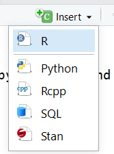
You can quickly insert chunks like these into your file with:
- the keyboard shortcut Ctrl + Alt + I (OS X: Cmd + Option + I)
- the Add Chunk command in the editor toolbar
- or by typing the chunk delimiters {r} and ```.
The most basic code chunk looks like so:

Other than our backticks ``` for code chunks that surround the code top and bottom, the only necessary piece is the specified language (r) placed between the curly brackets. This indicates that the language to read the code is R.
Fun fact: Other Programming Languages
Although we will (mostly) be using R in this workshop, it’s possible to use other programming or markup languages. For example, we have seen that we can use LaTeX code for equations. You can also use python too, and we (may) show an example with css. Other languages include: sql, julia, bash, and c, etc. It should be noted however, that some languages (like python) will require installing and loading additional packages.
Add a code chunk
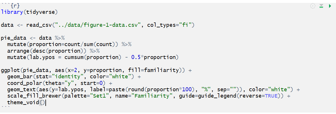
Ok, let’s add some code! Earlier, we added three images to our document. Now, images of our plots are great and all, but since R Markdown allows us to evaluate live code it would be more reproducible to use code chunks to display those plots. Like with our inline code, this assures that if there are any changes to the data, the plots update automatically. This also makes our life easier because when there’s a change we don’t have to re-generate plots, save them as images and then add them back in to our paper. This will potentially help prevent version errors as well! So we’re actually going to go ahead and convert a few of our plots to code chunks.
We’ll start by typing our our starting backticks & r between curly brackets. (in your own workflow you may want to add the ending three backticks as well so you don’t forget after adding your code):
Now, let’s open our plot-figure-1.r file in our code folder. Copy the code and paste it in between the two lines with backticks.
Tip:
There’s actually a button you can use in the RStudio menu to generate the code chunks automatically. Automatic code chunk generation is available for several other languages as well. Also, you can use the keyboard shortcut
ctrl+alt+Ifor Windows andcommand+option+Ifor Mac.
Run your code
Now, to check to make sure our code renders, we could click the “knit” button as we have been doing. However, with the code chunks we have other opportunities for rendering.
1) Knit button - knitting will automatically run the code in all code chunks
2) Run from Rmd file (green play button on the right top corner)
3) Run menu
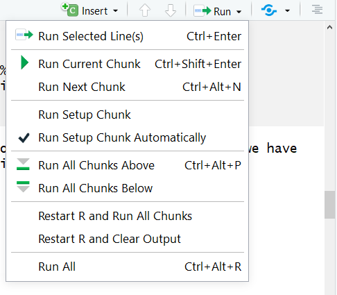
4) Keyboard shortcuts:
| Task | Windows & Linux | macOS |
|---|---|---|
| Run all chunks above | Ctrl+Alt+P | Command+Option+P |
| Run current chunk | Ctrl+Alt+C | Command+Option+C |
| Run current chunk | Ctrl+Shift+Enter | Command+Shift+Enter |
| Run next chunk | Ctrl+Alt+N | Command+Option+N |
| Run all chunks | Ctrl+Alt+R | Command+Option+R |
| Go to next chunk/title | Ctrl+PgDown | Command+PgDown |
| Go to previous chunk/title | Ctrl+PgUp | Command+PgUp |
Time to Knit!
Use one of the above options to run your code.
Name your code chunks
While not necessary for running your code, better practice is to give a name to each code chunk:
{r chunk-name}
Some things to keep in mind
- The chunk name is the only value other than r in the code chunk options that doesn’t require a tag (i.e. echo=FALSE)
- The chunk label has to be unique (i.e.you can’t use the the same name for multiple chunks)
We’ll see in a bit where this code chunk label comes in handy. But, for now let’s go back and give our first code chunk a name:
{r fig-1}
Tip: Don’t use spaces, periods or underscores in code chunk labels
Try to avoid spaces, periods (.), and underscores (_) in chunk labels and paths. If you need separators, you are recommended to use hyphens (-) instead. For example, setup-options is a good label, whereas setup.options and chunk 1 are bad; fig.path = ‘figures/mcmc-‘ is a good path for figure output, and fig.path = ‘markov chain/monte carlo’ is bad. See more at: https://yihui.org/knitr/options/
Code Chunk Options
There are over 50 different code chunk options!!! Obviously we will not go over all of them, but they fall into several larger categories including: code evaluation, text output, code style, cache options, plot output and animation. We’ll talk about a few options for code evaluation, text output and plot output specifically.
Again, The chunk name is the only value other than r in the code chunk options that doesn’t require a tag (i.e. the “= VALUE” part of option = VALUE). So these chunk options will always require a tag whose syntax looks like:
{r chunk-label, option = VALUE}
the option always follows the code chunk label (don’t forget to add a , after the label either).
Some common options:
eval = (logical or numeric) TRUE/FALSE to evaluate (or not) or a numeric value like c(1,3) (only evaluate expressions 1 and 3).
echo = (logical or numeric - following the same rules as above) whether to display source code or not.
warning = (logical) whether to display the warnings in the output (default:TRUE). FALSE will output warnings to the console only
include = (logical) whether to include the chunk output in the output document (default TRUE)
message = (logical) whether or not to display messages that appear when running the code (default TRUE)
CHALLENGE 9.2 - Rendering Codes
How will some hypothetical code render given the following options?
{r global-chunk-challenge, eval = TRUE, include = FALSE}SOLUTION
The expressions in the code chunk will be evaluated, but the outputed figures/plots will not be included in the knit document.
When might you want to use this?
If you need to calculate some value or do something on your dataset for a further calucation or plot, but the output is not important to be included in your paper narrative.
CHALLENGE 9.3 - add options to your code
Add the following options to your code:
echo = FALSE, message = FALSE, warning = FALSEWhat will this do?
SOLUTION
These options mean the source code will not be printed in the knit html document, messages from the code will not be printed in the knit html document, and warnings will not be printed in the knit html document (but will still output to the console). Plots, figures or whatever is printed by the code WILL show up in the final html document.
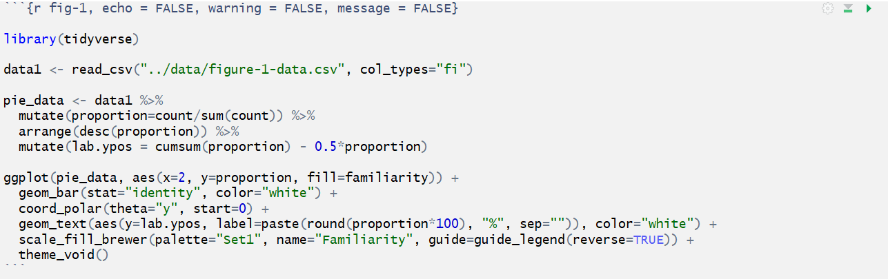
Time to Knit!
Make sure the options you added to your code chunk seem right.
Global Code Chunk Options:
With our first plot we set the options separately. However, we may end up with quite a few code chunks in our paper and it might be a lot of work to keep track of what options we’re using throughout the paper. We can automate setting options by adding a special code chunk at the beginning of the document. Then, each code chunk we add will refer to the options in this special when it runs.
To set global options that apply to every chunk in your file, call we will call knitr::opts_chunk$set() in a new code chunk right after our yaml header (name the new code chunk setup. Knitr will treat each option that add to this call as a global default. However, we will need to set the options for this code chunk in the first place! so we’ll use echo = FALSE. Then in the () after the knitr::opts_chunk$set() add the three options we used for our first code chunk.
Add to your file (with backticks):
{r setup, echo = FALSE}
knitr::opts_chunk$set(echo = FALSE, mesage = FALSE, warning = FALSE)
Alright! now let’s go back and remove the options we set in the individual code chunks & since we’ve set the global options in the document instead.
Time to Knit!
Again, let’s make sure our global options look right after knitting.
Tip: Yaml chunk options
We can also tweak some settings in our yaml which changes how code chunks are displayed. We’re not going to get into this in the workshop, but many of the same options you set in your global code chunk settings are also configurable in the yaml.
load our libraries and data “globally”
We can actually make our lives easier in one other way too. So far we’ve loaded the library tidyverse and dataframe data1 we need in the first code chunk. Now if we want to replace, say Figure 3 (which we will do next), we would load tidyverse and the data for Figure 3, meaning we would be loading tidyverse for a second time unecessarily. This is because once libraries and data are loaded they are available for the rest of the rmd document.
Instead, we can load libraries and data at the beginning of our document which makes it available for all other figures or calculations and lets us avoid the repitition. This also makes it easier for us to keep track of all the libraries and data we need to use in any given document. If anything needs to be tweaked, we don’t need to search through every code chunk in our rmd document to make a change.
Let’s add our libraries and data to a code chunk at the top of the document (and we can take this code out of Fig-1):
#load libraries
#tidyverse for plots
library(tidyverse)

#load data
#data for figure 1
data1 <- read_csv("../data/figure-1-data.csv", col_types="fi")
#data for table 1
table1 <- read_csv("../data/table.csv")
It’ll look like the following:
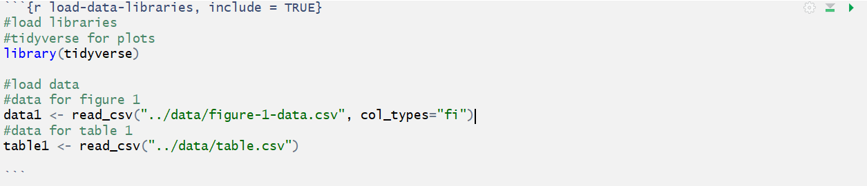
Time to Knit!
Make sure our code runs for Figure 1 now that we moved it around.
CHALLENGE 9.4 - Change the Fig 3 image to code
Now, let’s add the code to regenerate Figure 3 from the r script
plot-figure-3.rin thecodefolder:1) load the data for the figure in the designated code chunk at the top of our file.
2) Make a new code chunk where you want to replace the image for Figure 3.
3) Give it the name: fig-3
4) Don’t worry about options! we already set those in the global options.SOLUTION
from the
plot-figure-3.rr script, copy and paste the code to readfigure-3-data.csvtoload-data-libraries:
then, create a new code chunk at the spot in the paper we want figure 3 and paste in the rest of the code from
plot-figure-3.r:
Make sure the code chunk is namedfig-3
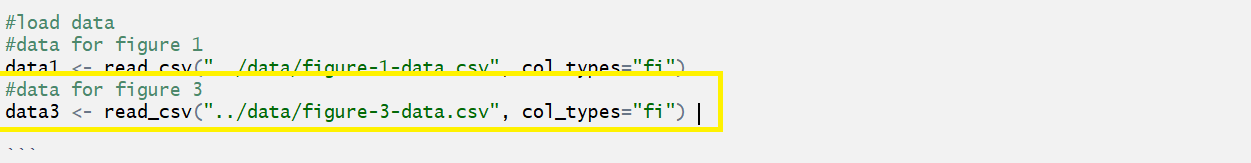
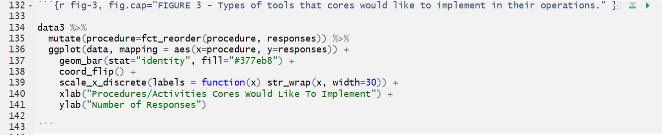
Time to Knit!
Make sure the code runs for Figure 3
Tip: Overiding global options
What if you want most of your code chunks to render with the same options (i.e. echo = FALSE), but you just have one or two chunks that you want to tweak the options on (i.e. display code with echo = TRUE)? Good news! The global options can be overwritten on a case by case basis in each individual code chunk.
CHALLENGE 9.5 (optional) global & individual code chunk options
How would appear in our html document if we knit a code chunk with the following options?
{r challenge-5, warning = TRUE, echo = TRUE}…considering the global chunk setting’s were as listed:
knitr::opts_chunk$set(echo = FALSE, include = FALSE)SOLUTION
In this case, the global settings are set so neither the code nor the output will display. However, the individual chunk reverses the echo setting so the code will display, and it also indicates that any warnings the code renders should output too. The outputs of the code would still not be displayed (include = FALSE) The hypothetical situation for this configuration may be for debugging while writing the rmd document.
Key Points
What is Knitr?
Inline code
Code chunks
Code chunk options
Global code chunk options
Knitr Syntax: Styling Code Outputs
Overview
Teaching: 35 min
Exercises: 5 minQuestions
How do I make better styled tables in R Markdown?
How do I add captions to code generated figures?
How do I consistently size and align images and figures?
How do I cross reference figures & tables?
Objectives
Create better styled tables
Add captions to code-generated figures, tables, images
Globally size and align images and figures
Use cross referencing
Create better tables in R Markdown
Our markdown table is formatted weirdly after knitting. Unfortunately, it isn’t possible to style tables created with basic markdown syntax. In order to create a table that is stylable, we need to save it as a dataframe and use a package function to style it. There are MANY packages that allow you to create tables in Rmd. See list (https://bookdown.org/yihui/rmarkdown-cookbook/table-other.html)
Restyle the table with kable
We will use kable to recreate our table. kable() is a function in the knitr package. kable() creates a basic stylable table.
1) load data & package in load-data-libraries chunk:
```{r load-data-libraries}
## ADD to existing libraries & data

#load knitr for kable table
library(knitr)

###

#load table 1 data
table1 <- read_csv("../data/table.csv")`
2) Delete the existing table (leave the caption for now)
3) create a new code chunk in place of the table, name it table-1
4) call kable() function on table1 dataframe
```{r table-1}
kable(table1)
Time to Knit!
Check to see if our table generated properly
your code chunk should output as so:
| Category | N |
|---|---|
| Poor sample quality from users/sample variability/limited biological material | 51 |
| Lack of well-trained principle investigators and lab members/Poor oversight | 45 |
| Poor experimental design: Lack of sufficient replicates/inadequate sample size/lack of adequate controls | 43 |
| Inadequate standardization of protocols or guidelines, and data analysis | 43 |
| Cost and time | 39 |
| Failure to leverage the core’s expertise/following the core’s advice/no consulting beforehand | 23 |
| Inadequate documentation of experiments/data management | 19 |
| Instruments: maintenance, upgrades, changes | 15 |
| Responses that could not be assigned to a category | 11 |
Note: Styling kable tables
You can use the argument
formatto specify betweenhtml,latex,pipe, orrststyles. This can also be set in the global options withknitr.table.format. For additional styling, there is a function calledkable_styling()to change the look of your kable tables. https://www.rdocumentation.org/packages/kableExtra/versions/1.3.1/topics/kable_styling
Note: Other table packages
Even though we can do a bit more styling with
kable(), it’s still pretty basic. To do more complex tables,kableExtrapackage was developed. This especially allows more control over formatting. There are other multiple other packages as well that help with table formattingofficerfor Word andxtableare two examples. officer: https://www.rdocumentation.org/packages/officer/versions/0.3.15 https://bookdown.org/yihui/rmarkdown-cookbook/table-other.html
Note: Styling Kable tables
You can use the argument
formatto specify betweenhtml,latex,pipe, orrststyles. This can also be set in the global options withknitr.table.format. For additional styling, there is a function calledkable_styling()to change the look of your kable tables. https://www.rdocumentation.org/packages/kableExtra/versions/1.3.1/topics/kable_styling
Add captions to code-generated tables & plots
Also, we learned how to add captions to images earlier on, but now, how do we add captions to the code-generated plots and the new table we just added? It is a little different between tables and code-generated plots/images.
Add captions to code-generated tables
Ok, let’s start with the table. The kable() function has an argument called caption.
1) cut the orignial table caption from it’s spot in the paper
2) add to the kable function caption = and paste the caption in between "s
caption="Table 1. Major challenges to rigor observed in shared resources"
code will look like so:
```{r table-1}
kable(table1, caption="Table 1. Major challenges to rigor observed in shared resources")
Time to Knit!
Did the caption output for Table 1?
Hint: it will appear above the table.
Add captions to code-generated plots, figures & images
To add captions for Figure 1 and 3 we’re going to go back to our favorite: code chunk options. Anytime after defining the code chunk name we can add the chunk option: fig.cap = (so either before or after the other options, order doesn’t matter). Notice that the syntax is slightly different than our other options but it has the same = . Instead of indicating TRUE/FALSE however, we can type our caption right after the = in quotes fig.cap = "". NOTE: we are adding this to the code chunk options, NOT as an argument to the code like for the table.
1) type in fig.cap = "" after the chunk label (and a comma)
2) paste or type in the caption
FIGURE 1 - Knowledge and awareness of the current NIH guidelines on rigor and reproducibility.
Your code chunk options should now look like this:
{r fig-1, fig.cap="FIGURE 1 - Knowledge and awareness of the current NIH guidelines on rigor and reproducibility."}
#code for figure 1 here
Time to Knit!
Check to see if the caption for Figure 1 appeared
CHALLENGE 9.1 - add a caption for Figure 3
Add the caption to the code for Figure 3:
FIGURE 3 - Types of tools that cores would like to implement in their operations.SOLUTION
{r fig-3, fig.cap="FIGURE 3 - Types of tools that cores would like to implement in their operations." }
Time to Knit!
Check to see if caption for Figure 3 appeared
Globally & Automatically align & size plots/figures
We changed the sizing of our images in a previous episode. However, instead of changing the sizes one-by one, we can do it within our knitr::opts_chunk$set settings in our setup code chunk.
Automatically size figures & images
We can size with a number of inches, percentage of the original image size, or pixels (in some cases). The default for inches is 7in height and width for code-generated figures, plots & images (knitr) versus it’s 5in height by 7in width for markdown generated images (rmarkdown).
There is no default for perentages because the default size is inches. When using percentages it’s important to note that % refers to the percent of the HTML container. So images are sized in relation to their original size, but in relation to the html document size. For example, if the block of text on a webpage is 1000px wide then resizing at 20% width means the image will be 200px in width.
Option options for resizing
Two options fig. and out.. out. is more expansize than fig. both in how size can be defined and what kind of figures/plots/images it can be applied to.
fig.width along with fig.height, ONLY applies to R-generated figures defined within a code chunk. It changes the width of the images based on the specifications which can be defined in inches & percentage.
fig.height along with fig.width, ONLY applies to R-generated figures defined within a code chunk. It changes the height of the images based on the specifications which can be defined in inches & percentage.
out.width along with out.height, can be applied to any type of graphic defined within a code chunk. It changes the width of the images based on the specifications which can be defined in inches, percentage & number of pixels.
out.height along with out.width, can be applied to any type of graphic defined within a code chunk. It changes the height of the images based on the specifications which can be defined in inches, percentage & number of pixels.
We want to be inclusive of the images in our Rmd file so we will use out.width & out.height which offers more flexibility. Also, we previously sized the images to 50%, but that was a bit small, so let’s try 60% instead.
Add to (before or after) the other options, in the global code chunk:
knitr::opts_chunk$set(out.width="60%", out.height="60%", echo = FALSE, message = FALSE, warning = FALSE)
Time to Knit!
See how our images re-sized.
Oh no, Fig 2 isn’t aligning! Unfortunately, the settings ONLY apply to knitr-rendered code chunks, but our Figure 2 is still just a rmarkdown-styled image.
We can add the Fig 2 .jpg to a code chunk instead:
1) create a new code chunk and name the it fig-2
2) copy and paste the caption between quotes with the fig.cap="" option.
3) use include_graphics() function from the knitr package (alternatively can use syntax knitr::include_graphics()) if you haven't loaded the package.
4) Add the file path in quotes between the () of include_graphics().
{r fig-2, eval = FALSE, echo = TRUE, fig.cap="FIGURE 2 - Lack of requests for rigor and reproducibility documentation by users of shared resources."}
include_graphics("../figs/fig2_paper.jpg")
Time to Knit!
Check to see if all images re-sized
Automatically align code chunk outputs
To automatically & globally align code chunk outputs like we did with sizing, add to the setup code chunk:
fig.align = "center"
so the whole chunk will look like so:
knitr::opts_chunk$set(fig.align = "center", out.width="60%", out.height="60%", echo = FALSE, message = FALSE, warning = FALSE)
Time to Knit!
Check to see if all images and figures were aligned to the center
Cross-referencing (optional)
from bookdown.org:
Cross-referencing is a useful way of directing your readers through your document, and can be automatically done within R Markdown. While this has been explained in Chapter 2 from the bookdown book, we want to present a brief summary below.
To use cross-references, you will need:
- A bookdown output format: Cross-referencing is not provided directly within the base rmarkdown package, but is provided as an extension in bookdown (Xie 2020c). We must therefore use an output format from bookdown (e.g., html_document2, pdf_document2, and word_document2, etc.) in the YAML output field.
- A caption to your figure (or table): Figures without a caption will be included directly as images and will therefore not be a numbered figure.
- A labeled code chunk: This provides the identifier for referencing the figure generated by the chunk.
After these conditions are met, we can make cross-references within the text using the syntax \@ref(type:label), where label is the chunk label and type is the environment being referenced (e.g. tab, fig, or eqn). An example is provided below:
We’ve already installed bookdown in our setup steps at the beginning of the workshop, but we need to make sure to load the bookdown library.
Add into your load-data-libraries code chunk:
#load bookdown for cross-referencing
library(bookdown)
We also need to change the output in the yaml to a bookdown specification so, change the output yaml in the yaml to the following(the rest stays the same.):
...
ouput:
  bookdown::html_document2:
...
Now to add cross referencing:
This is the syntax for a cross-reference link:
\@ref(type:label)
the \@ref will always remain the same. We will edit type and label
type options:
- tab : for tables
- fig : for figures
- eqn : for equations
label is replaced with the chunk label of the code chunk figure/table/equation you want to link to.
Let’s try this out on our paper:
1) Find or search for the note: (See Table 1) in the Core Implementation section.
2) To add a cross reference link we will replace the “Table 1” text with:
\@ref(tab:table-1)
we will replace type with tab and label with table-1.
Time to Knit!
Check to see if the cross reference link for Table 1 appeared. Notice what happens when you click the link.
CHALLENGE 9.2: Add a Cross Reference to Figure 2
Search for or find in the text: “(See Figure 2)” in the “Strategies for Improving R&R sub section: Make this into a cross reference link.
SOLUTION
\@ref(fig:fig-2)
*Note adding crossing referencing re-names the figures, so should take the figure numbering out.
Time to Knit!
Check to see if the cross reference links appeared
Styling conclusions
There are a plethora of options for styling, from additional bookdown options, to things you can edit in the yaml (including adding themes to style text), and adding your own custom css style sheets. Explore more on your own!
Key Points
Use kable() to create tables from dataframes
add captions to figures and images generated by code chunks
Set global chunk settings to automatically size & align outputs
Use bookdown to enable cross referencing
Publishing a Report
Overview
Teaching: 20 min
Exercises: 10 minQuestions
How to change the output folder for your rendered document?
How to publish your report on RPubs?
How to use Github to publish your document as a webpage?
Objectives
Explore Different methods for publishing your paper
Changing the behavior of the Knit Button
In episode 2 we said we would show you later on how to change the behavior of the knit button so you could conform to best practices for organizing your R project. We would prefer to save the output to the results folder instead of the code folder because it’s best practice to save your outputs (whether knit rmd documents, the outputs of r scripts, or cleaned data) in a folder separate from your ‘raw’ code and data. That way for instance, you can avoid deleting or saving over your raw data and you can save different iterations of your outputs without worry.
R Studio provides options to set the output type and a few other things but does not let the user select a destination folder for knitr output. But users CAN however add code to the yaml which allows finer control of the behavior of the knit button. Once you’ve set directives in the header YAML section of your R-markdown file everytime you hit ‘knit’, R Studio follows your customized directives as it processes the code to render your output.
So, let’s copy and paste the the following to our yaml header (placing the code after the bibliography and/or csl section should work.):
...
...
knit: (function(rmdfile, ...) { rmarkdown::render(rmdfile, output_dir='../results') })
---
What’s going on in this YAML code we’re adding:
knit we are changing the behavior of the knit function by defining our own:
function(rmdfile, …) as stated above we are defining our own function by calling function() so we can re-design what happens when we hit ‘knit’. rmdfile is the main parameter required for our render function. This just means that the input file is ‘this’ file - the .rmd file we are kniting.
rmarkdown::render When you click the knit button R-Studio runs rmarkdown:render.
Typing ?rmarkdown::render in the console will bring up further information about the rmarkdown:render function. We will be using two arguments of rmarkdown::render.
- input: The file we’re feeding the function. We already determined this is
rmdfileor ‘this’ document. - output_dir: designates which folder we want to save the knit document to (relative path). In our case we know this is the
resultsfolder so we use..to go back to our root directory (from the code folder). The “default” folder is the folder where your rmd file is saved, so any ‘directions’ you give by indicating a relative path will be from the folder where the rmd file is to the folder where you want to save the html rendered document.
Time to Knit!
Check if your html file was saved to the
resultsfolder.
Rendering R Markdown script
Once you have your .Rmd document refined and the Knit output looks good it is ready to publish. When using RStudio the simplest option is to publish to Rpubs.com. Rpubs is a bare-bones web hosting service created for the sole purpose of hosting RMarkdown documents. It provides no other services— no support for search, collaboration, persistent identifers, or versioning. But, it is the simplest and most direct way of getting your RMarkdown document published on the web directly from RStudio. For a more full-featured hosting service consider GitHub and GitHub Pages, described later.
Notice the “Publish” button in the upper right corner of your Knit output. Click this to publish to Rpubs. This is where you’ll need an Rpubs account as mentioned in setup for this workshop.
Click the publish button

and you’ll be presented with the following panels:
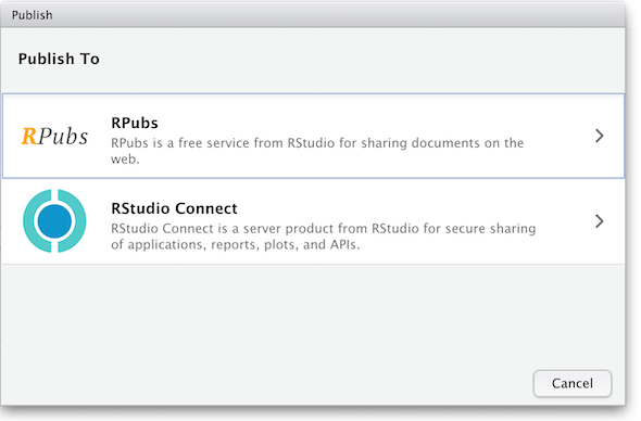 (The other option in the dialog box, RStudio Connect, is a standalone publishing platform for teams to share content. It requires purchase to host and use.)
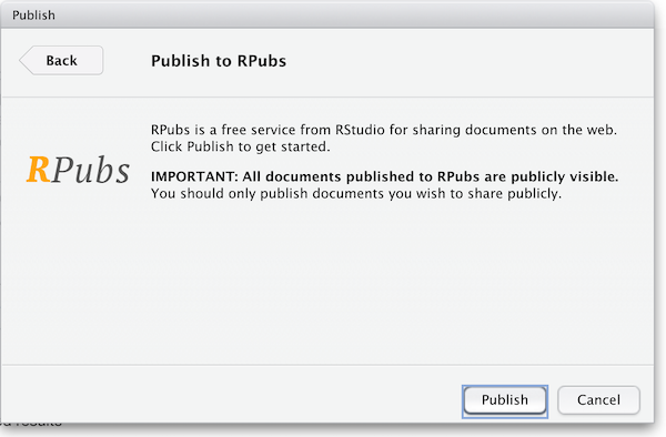
The first time you publish, RStudio will likely ask if you want to install some needed packages; say yes. RStudio will then open up a web browser to allow you sign in to rpubs.com.
At the end of the publish process your paper will be live on the internet
with a URL similar to: https://rpubs.com/yourname/678624
RStudio also saves an HTML version of your knit document to your local file system. Look for it in the results
directory in the same directory as the R-markdown file in your R-Studio project directory.
This html document is self-contained and highly portable. Images are encoded directly into the HTML so you can easily move it to any web hosting you have available.
Publishing as website on GitHub*
Another, better, but slightly more involved option for publishing an RMarkdown document on the web is to use GitHub and GitHub Pages. It is out of the scope of this lesson to use GitHub, but briefly, GitHub is a widely-used version control and collaboration system. RStudio has built-in support for GitHub: in the upper right panel of your RStudio window, look for the Git tab, which allows you to sync your RMarkdown project with a remote repository stored on github.com. To enable publishing to GitHub Pages, go to the Settings page of your repository on GitHub and select a branch (“branch” is a repository term) to publish. Name your main RMarkdown file index.Rmd, and render it to HTML as index.html. With GitHub Pages enabled on your repository, the HTML file in your repository at https://github.com/myusername/myrepo/index.html will appear on the web as https://myusername.github.io/.
Other document types
When you create a new R-markdown file in R Studio you are presented with a choice of Output Formats:
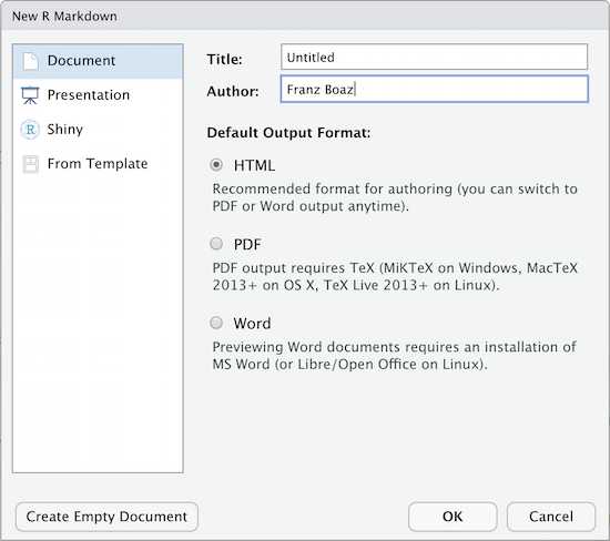
For the purposes of this workshop we’re using HTML as the output format but other types are available. You can render your R Markdown as a document, a presentation or a Shiny app. With the default installation of R-Studio HTML output is most likely to work. Other formats may require additional R packages and/or code libraries be installed on your computer. R Studio also has a templating system to help with creating R Markdown files with common elements, YAML metadata and rendering instructions. This can be very helpful for example if you want to create a weekly or monthly report documenting an ongoing experiment, study or other changing data.
Key Points
Define a new function for
knitin the yaml to change your outputsR-Studio lets you Knit and Publish to R-pubs
Github has Github Pages to publish work as a free webpage