Knitr Syntax: Inline Code & Code Chunks
Overview
Teaching: 40 min
Exercises: 15 minQuestions
What is “Knitr”?
When would I want to add inline code?
How to add inline code?
When would I want to use code chunks?
How do I add code chunks?
Objectives
Understand the basic functions of Knitr
Learn how to add inline code to your document
Learn how to add code chunks to your document
Distinguish when inline code vs. code chunks would be appropriate
Understand how to change the output characteristics of code chunks
What is Knitr?
Knitr is the engine in RStudio which creates the “dynamic” part of R markdown reports. It’s specifically a package that allows the integration of R code into the html, word, pdf, or LaTex document you have specified as your output for r markdown. It utilizes Literate Programming to make research more reproducible. There are two main ways to process code with Knitr in R Markdown documents:
- Inline code
- Code Chunks
Adding Inline code
Inline code is best for calculating simple expressions integrated into your narrative. For example, use inline code to calculate an error margin or summary statistic, such as # of observations, of your dataframe in your results section. One of the benefits of using this method is if something about your data set changes (like leaving out NAs or null values) the code will automatically update the calcuation specified.
We’re going to go ahead and change the LaTex code we used to input the error margin and calculate it dynamically using r code. So, instead of $ \pm 3 \% $ to display our error margin as +/-3%, let’s add this:
`r round(1.96*0.5*(1-0.5)/sqrt(243)*100)`%
Notice how we put the % sign after the ticks. In this case the percentage sign should be plain text. If we had put it inside the ending backtick (`) r would have attempted to calculate the modulo since that’s what that symbol stands for in R.
Time to Knit!
See that inline code evaluates to calculate the error margin of +/- 3%.
Where else can we add inline code? We can replace observation counts!
i.e. “There are #r nrow(my_data) individuals who completed the survey”
Now, we’re going to find one such example in our data frame and convert a static number or equation to inline code. In our paper text we read “a total of 243 individuals from 21 countries completed this section.” Here we can use inline r code to calculate the total responses instead of typing it in.
However, because we don’t have access to the original dataset (and thus only aggregate counts) we can’t use nrow() to count our number of observations. we will count the column count in our data1 dataframe which sums the responses relating to how familiar respondents are with current NIH guidelines on reproducibility and is used to create Fig 1. We will use r sum(data1$count) in between the tick marks instead to total the count for each level of familiarity (“Very Aware”, “Somewhat Aware”, “Completely Unaware”).
We will add the inline code to the sentence in question:
a total of `r sum(data1$count)` individuals from 21 countries completed this section.
Output:
"a total of 242 individuals from 21 countries completed this section."
Time to Knit!
See that the r inline code evaluates in the sentence.
Oh! Wow we were off on out total count by one anyway, good thing we added this inline code!
Tip: Inline code cannot span lines
You need to be sure that these in-line bits of code aren’t split across lines in your document. Otherwise you’ll just see the raw code and not the result that you want.
CHALLENGE 9.1 - Converting a static number to inline code
There are two more spots in the paper where the count 243 was stated (search ‘243’ or look just around the paragraph we just edited) Find both and replace with code. What part of the paper is that?
SOLUTION
1. the margin of error is ±`r round(1.96*0.5*(1-0.5)/sqrt(sum(data1$count))*100)`%Note: since this we just added inline code to calculate the error margin, we can just add this snippet to count the total respondents, this means we only need to substitute
sum(data1$count)for 243 (and don’t need to add the backticks andra second time.2. sample size $n=`r sum(data1$count)`$Note: Look at that! you can add r inline code in LaTex formatting, it evaluates the r code and then displays in LaTex format!
Time to Knit!
Let’s make sure everything looks right for our inline code
Inserting Code Chunks
Code chunks are better when you need to do something more sophisticated with your code, such as building plots or tables. There is also syntax which allows you to change how that code gets rendered. We’ll learn more about that as we walk through the “anatomy” of a code chunk.
Basic Anatomy of the Code Chunk
You can quickly insert chunks like these into your file with:
- the keyboard shortcut Ctrl + Alt + I (OS X: Cmd + Option + I)
- the Add Chunk command in the editor toolbar
- or by typing the chunk delimiters {r} and ```.
The most basic code chunk looks like so:

Other than our backticks ``` for code chunks that surround the code top and bottom, the only necessary piece is the specified language (r) placed between the curly brackets. This indicates that the language to read the code is R.
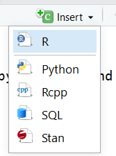
Fun fact: Other Programming Languages
Although we will (mostly) be using R in this workshop, it’s possible to use other programming or markup languages. For example, we have seen that we can use LaTeX code for equations. You can also use python too, and we (may) show an example with css. Other languages include: sql, julia, bash, and c, etc. It should be noted however, that some languages (like python) will require installing and loading additional packages.
Add a code chunk
Ok, let’s add some code! Earlier, we added three images to our document. Now, images of our plots are great and all, but since R Markdown allows us to evaluate live code it would be more reproducible to use code chunks to display those plots. Like with our inline code, this assures that if there are any changes to the data, the plots update automatically. This also makes our life easier because when there’s a change we don’t have to re-generate plots, save them as images and then add them back in to our paper. This will potentially help prevent version errors as well! So we’re actually going to go ahead and convert a few of our plots to code chunks.
We’ll start by typing our our starting backticks & r between curly brackets. (in your own workflow you may want to add the ending three backticks as well so you don’t forget after adding your code):
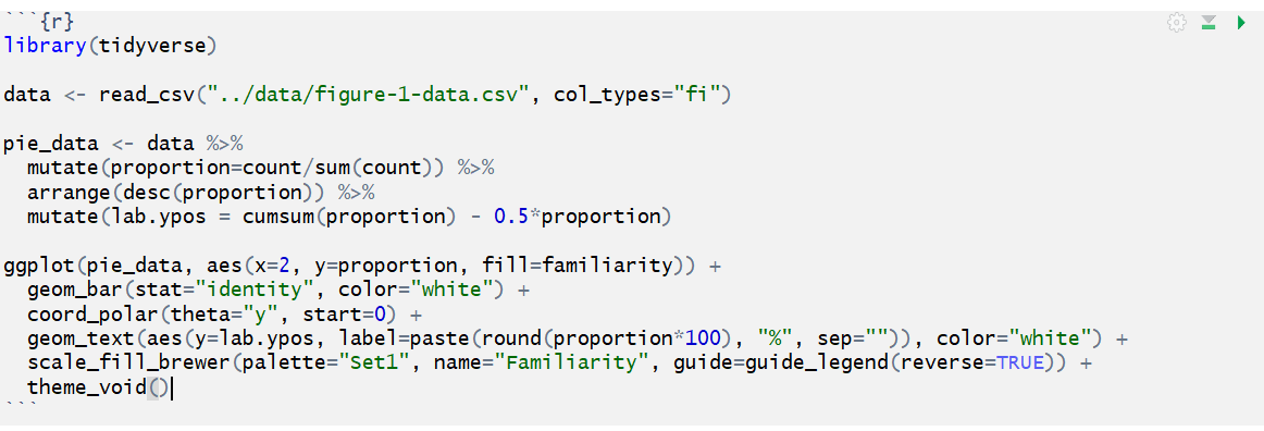
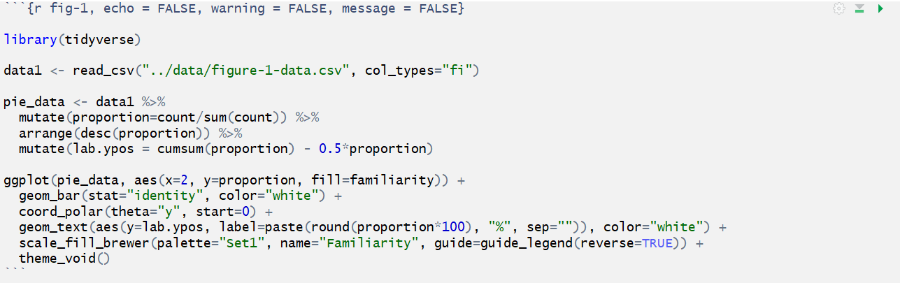
Now, let’s open our plot-figure-1.r file in our code folder. Copy the code and paste it in between the two lines with backticks.
Tip:
There’s actually a button you can use in the RStudio menu to generate the code chunks automatically. Automatic code chunk generation is available for several other languages as well. Also, you can use the keyboard shortcut
ctrl+alt+Ifor Windows andcommand+option+Ifor Mac.
Run your code
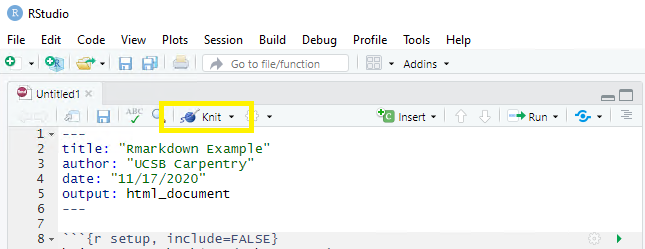
Now, to check to make sure our code renders, we could click the “knit” button as we have been doing. However, with the code chunks we have other opportunities for rendering.
1) Knit button - knitting will automatically run the code in all code chunks
2) Run from Rmd file (green play button on the right top corner)
3) Run menu
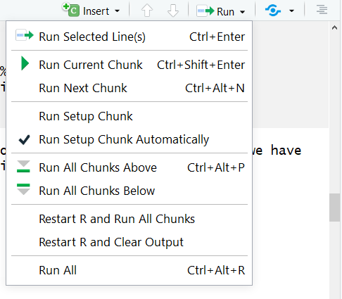
4) Keyboard shortcuts:
| Task | Windows & Linux | macOS |
|---|---|---|
| Run all chunks above | Ctrl+Alt+P | Command+Option+P |
| Run current chunk | Ctrl+Alt+C | Command+Option+C |
| Run current chunk | Ctrl+Shift+Enter | Command+Shift+Enter |
| Run next chunk | Ctrl+Alt+N | Command+Option+N |
| Run all chunks | Ctrl+Alt+R | Command+Option+R |
| Go to next chunk/title | Ctrl+PgDown | Command+PgDown |
| Go to previous chunk/title | Ctrl+PgUp | Command+PgUp |
Time to Knit!
Use one of the above options to run your code.
Name your code chunks
While not necessary for running your code, better practice is to give a name to each code chunk:
{r chunk-name}
Some things to keep in mind
- The chunk name is the only value other than r in the code chunk options that doesn’t require a tag (i.e. echo=FALSE)
- The chunk label has to be unique (i.e.you can’t use the the same name for multiple chunks)
We’ll see in a bit where this code chunk label comes in handy. But, for now let’s go back and give our first code chunk a name:
{r fig-1}
Tip: Don’t use spaces, periods or underscores in code chunk labels
Try to avoid spaces, periods (.), and underscores (_) in chunk labels and paths. If you need separators, you are recommended to use hyphens (-) instead. For example, setup-options is a good label, whereas setup.options and chunk 1 are bad; fig.path = ‘figures/mcmc-‘ is a good path for figure output, and fig.path = ‘markov chain/monte carlo’ is bad. See more at: https://yihui.org/knitr/options/
Code Chunk Options
There are over 50 different code chunk options!!! Obviously we will not go over all of them, but they fall into several larger categories including: code evaluation, text output, code style, cache options, plot output and animation. We’ll talk about a few options for code evaluation, text output and plot output specifically.
Again, The chunk name is the only value other than r in the code chunk options that doesn’t require a tag (i.e. the “= VALUE” part of option = VALUE). So these chunk options will always require a tag whose syntax looks like:
{r chunk-label, option = VALUE}
the option always follows the code chunk label (don’t forget to add a , after the label either).
Some common options:
eval = (logical or numeric) TRUE/FALSE to evaluate (or not) or a numeric value like c(1,3) (only evaluate expressions 1 and 3).
echo = (logical or numeric - following the same rules as above) whether to display source code or not.
warning = (logical) whether to display the warnings in the output (default:TRUE). FALSE will output warnings to the console only
include = (logical) whether to include the chunk output in the output document (default TRUE)
message = (logical) whether or not to display messages that appear when running the code (default TRUE)
CHALLENGE 9.2 - Rendering Codes
How will some hypothetical code render given the following options?
{r global-chunk-challenge, eval = TRUE, include = FALSE}SOLUTION
The expressions in the code chunk will be evaluated, but the outputed figures/plots will not be included in the knit document.
When might you want to use this?
If you need to calculate some value or do something on your dataset for a further calucation or plot, but the output is not important to be included in your paper narrative.
CHALLENGE 9.3 - add options to your code
Add the following options to your code:
echo = FALSE, message = FALSE, warning = FALSEWhat will this do?
SOLUTION
These options mean the source code will not be printed in the knit html document, messages from the code will not be printed in the knit html document, and warnings will not be printed in the knit html document (but will still output to the console). Plots, figures or whatever is printed by the code WILL show up in the final html document.
Time to Knit!
Make sure the options you added to your code chunk seem right.
Global Code Chunk Options:
With our first plot we set the options separately. However, we may end up with quite a few code chunks in our paper and it might be a lot of work to keep track of what options we’re using throughout the paper. We can automate setting options by adding a special code chunk at the beginning of the document. Then, each code chunk we add will refer to the options in this special when it runs.
To set global options that apply to every chunk in your file, call we will call knitr::opts_chunk$set() in a new code chunk right after our yaml header (name the new code chunk setup. Knitr will treat each option that add to this call as a global default. However, we will need to set the options for this code chunk in the first place! so we’ll use echo = FALSE. Then in the () after the knitr::opts_chunk$set() add the three options we used for our first code chunk.
Add to your file (with backticks):
{r setup, echo = FALSE}
knitr::opts_chunk$set(echo = FALSE, mesage = FALSE, warning = FALSE)
Alright! now let’s go back and remove the options we set in the individual code chunks & since we’ve set the global options in the document instead.
Time to Knit!
Again, let’s make sure our global options look right after knitting.
Tip: Yaml chunk options
We can also tweak some settings in our yaml which changes how code chunks are displayed. We’re not going to get into this in the workshop, but many of the same options you set in your global code chunk settings are also configurable in the yaml.
load our libraries and data “globally”
We can actually make our lives easier in one other way too. So far we’ve loaded the library tidyverse and dataframe data1 we need in the first code chunk. Now if we want to replace, say Figure 3 (which we will do next), we would load tidyverse and the data for Figure 3, meaning we would be loading tidyverse for a second time unecessarily. This is because once libraries and data are loaded they are available for the rest of the rmd document.
Instead, we can load libraries and data at the beginning of our document which makes it available for all other figures or calculations and lets us avoid the repitition. This also makes it easier for us to keep track of all the libraries and data we need to use in any given document. If anything needs to be tweaked, we don’t need to search through every code chunk in our rmd document to make a change.
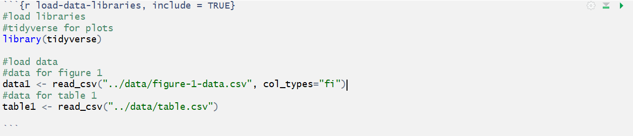
Let’s add our libraries and data to a code chunk at the top of the document (and we can take this code out of Fig-1):
#load libraries
#tidyverse for plots
library(tidyverse)

#load data
#data for figure 1
data1 <- read_csv("../data/figure-1-data.csv", col_types="fi")
#data for table 1
table1 <- read_csv("../data/table.csv")
It’ll look like the following:
Time to Knit!
Make sure our code runs for Figure 1 now that we moved it around.
CHALLENGE 9.4 - Change the Fig 3 image to code
Now, let’s add the code to regenerate Figure 3 from the r script
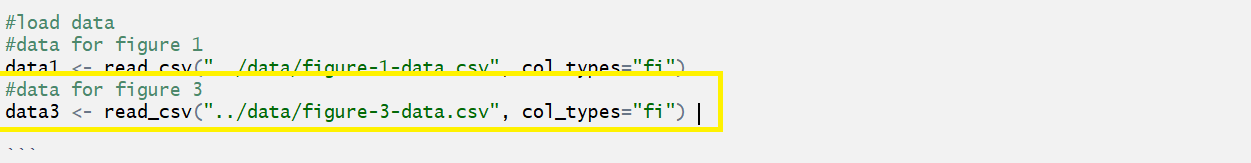
plot-figure-3.rin thecodefolder:1) load the data for the figure in the designated code chunk at the top of our file.
2) Make a new code chunk where you want to replace the image for Figure 3.
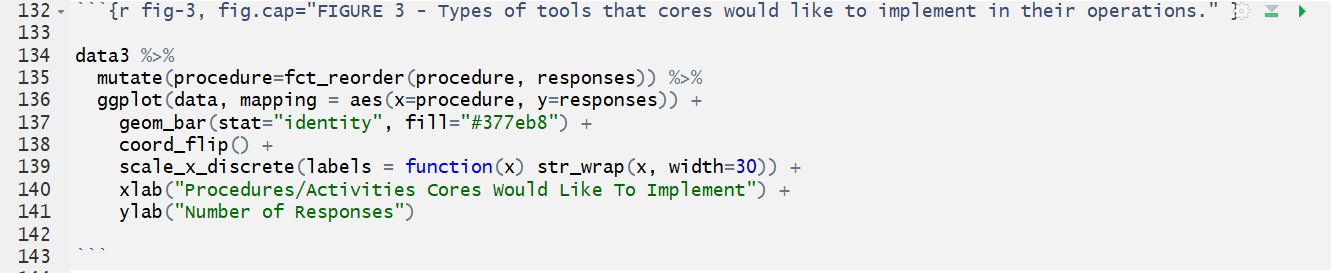
3) Give it the name: fig-3
4) Don’t worry about options! we already set those in the global options.SOLUTION
from the
plot-figure-3.rr script, copy and paste the code to readfigure-3-data.csvtoload-data-libraries:
then, create a new code chunk at the spot in the paper we want figure 3 and paste in the rest of the code from
plot-figure-3.r:
Make sure the code chunk is namedfig-3
Time to Knit!
Make sure the code runs for Figure 3
Tip: Overiding global options
What if you want most of your code chunks to render with the same options (i.e. echo = FALSE), but you just have one or two chunks that you want to tweak the options on (i.e. display code with echo = TRUE)? Good news! The global options can be overwritten on a case by case basis in each individual code chunk.
CHALLENGE 9.5 (optional) global & individual code chunk options
How would appear in our html document if we knit a code chunk with the following options?
{r challenge-5, warning = TRUE, echo = TRUE}…considering the global chunk setting’s were as listed:
knitr::opts_chunk$set(echo = FALSE, include = FALSE)SOLUTION
In this case, the global settings are set so neither the code nor the output will display. However, the individual chunk reverses the echo setting so the code will display, and it also indicates that any warnings the code renders should output too. The outputs of the code would still not be displayed (include = FALSE) The hypothetical situation for this configuration may be for debugging while writing the rmd document.
Key Points
What is Knitr?
Inline code
Code chunks
Code chunk options
Global code chunk options