Getting Started with R Markdown

Overview

Teaching: 15 min
Exercises: 10 min

Questions

• How to find your way around RStudio?

• How to start an R Markdown document in Rstudio?

• How is an R Markdown document configured & what is our workflow?

Objectives

• Key Functions in Rstudio

• Learn how to start an R markdown document

• Understand the workflow of an R Markdown file

Getting Around RStudio

Throughout this lesson, we’re going to teach you some of the fundamentals of using R Markdown as part of your RStudio workflow.

We’ll be using RStudio: a free, open source R Integrated Development Environment (IDE). It provides a built in editor, works on all platforms (including on servers) and provides many advantages such as integration with version control and project management.

This lesson assumes you already have a basic understanding of R and RStudio but we will do a brief tour of the IDE, review R projects and the best practices for organizing your work, and how to install packages you may want to use to work with R Markdown.

Basic layout

When you first open RStudio, you will be greeted by three panels:

• The interactive R console/Terminal (entire left)
• Environment/History/Connections (tabbed in upper right)
• Files/Plots/Packages/Help/Viewer (tabbed in lower right)

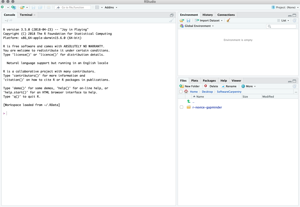
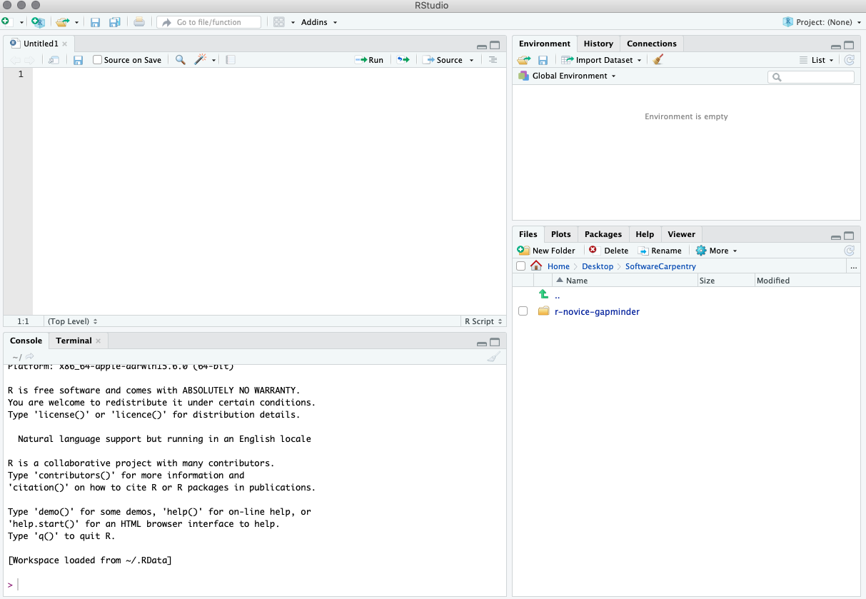
Once you open files, such as .Rmd files or .R files, an editor panel will also open in the top left.

Working in an R Project

The scientific process is naturally incremental, and many projects start life as random notes, some code, then a manuscript, and eventually everything is a bit mixed together.

Managing your projects in a reproducible fashion doesn't just make your science reproducible, it makes your life easier.

— Vince Buffalo (@vsbuffalo) April 15, 2013

Most people tend not to think about how to organize their files which may result in something like this:

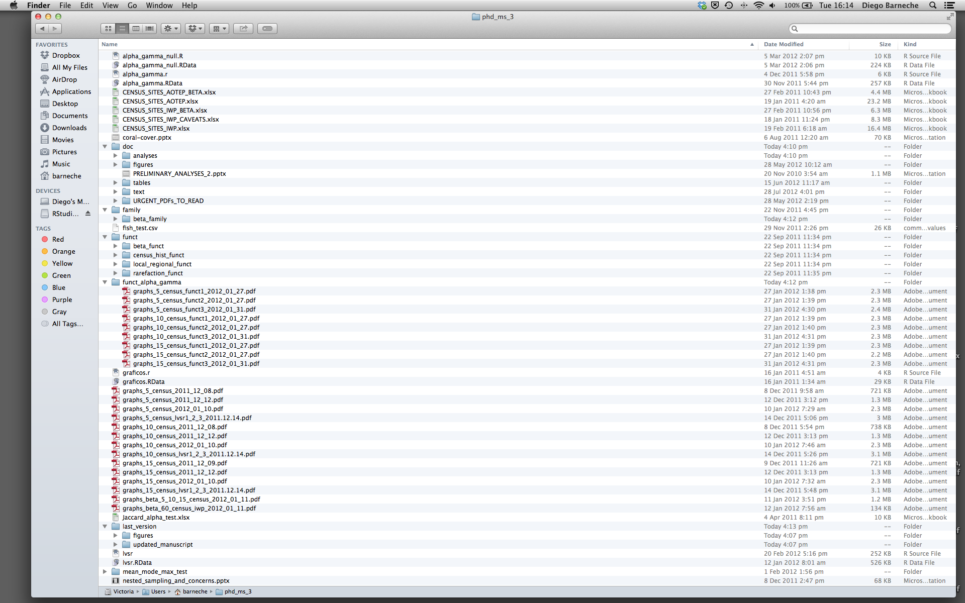
There are many reasons why we should ALWAYS avoid this:

1. It is really hard to tell which version of your data is the original and which is the modified;
2. It gets really messy because it mixes files with various extensions together;
3. It probably takes you a lot of time to actually find things, and relate the correct figures to the exact code that has been used to generate it;

A good project layout will ultimately make your life easier:

• It will help ensure the integrity of your data;
• It makes it simpler to share your code with someone else (a lab-mate, collaborator, or supervisor);
• It allows you to easily upload your code with your manuscript submission;
• It makes it easier to pick the project back up after a break.

A possible solution

Fortunately, there are tools and packages which can help you manage your work effectively.

One of the most powerful and useful aspects of RStudio is its project management functionality. We’ll be using an R project today to complement our R Markdown document and bundle all the files needed for our paper into a self-contained, reproducible project. After opening the project we’ll review good ways to organize your work.

The simplest way to open an RStudio project once it has been created is to click through your file system to get to the directory where it was saved and double click on the .Rproj file. This will open RStudio and start your R session in the same directory as the .Rproj file. All your data, plots and scripts will now be relative to the project directory. RStudio projects have the added benefit of allowing you to open multiple projects at the same time each open to its own project directory. This allows you to keep multiple projects open without them interfering with each other.

CHALLENGE 2.1 - Opening a Project in RStudio

Open an RStudio project through the file system

1. Exit RStudio.
2. Navigate to the directory where you downloaded & unzipped the zip folder for this workshop
3. Double click on the .Rproj file in that directory.

SOLUTION

double click on the RMarkdown_Workshop.Rproj to automatically open in R Studio

Best practices for project organization

Although there is no “best” way to lay out a project, there are some general principles to adhere to that will make project management easier:

Treat data as read only

This is probably the most important goal of setting up a project. Data is typically time consuming and/or expensive to collect. Working with them interactively (e.g., in Excel) where they can be modified means you are never sure of where the data came from, or how it has been modified since collection. It is therefore a good idea to treat your data as “read-only”.

Data Cleaning

In many cases your data will be “dirty”: it will need significant preprocessing to get into a format R (or any other programming language) will find useful. This task is sometimes called “data munging”. Storing these scripts in a separate folder, and creating a second “read-only” data folder to hold the “cleaned” data sets can prevent confusion between the two sets.

Treat generated output as disposable

Anything generated by your scripts should be treated as disposable: it should all be able to be regenerated from your scripts.

There are lots of different ways to manage this output. Having an output folder with different sub-directories for each separate analysis makes it easier later. Since many analyses are exploratory and don’t end up being used in the final project, and some of the analyses get shared between projects.

Use Rmd files to combine code/analysis and narrative

Rmd combines the power of R code and analysis with narratives describing methods and results. Keeping your code and narrative in the same document increases reproducibility by bundling paper components together; decreasing the amount of work you, your collaborators, and your audience has to do to search for different components of your project: raw data, analysis and plots, narrative, and citations.

Tip: Good Enough Practices for Scientific Computing

Good Enough Practices for Scientific Computing gives the following recommendations for project organization:

1. Put each project in its own directory, which is named after the project.
2. Put text documents associated with the project in the doc directory.
3. Put raw data and metadata in the data directory, and files generated during cleanup and analysis in a results directory.
4. Put source for the project’s scripts and programs in the src directory, and programs brought in from elsewhere or compiled locally in the bin directory.
5. Name all files to reflect their content or function.

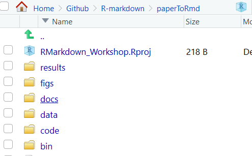
For this project, we used the following setup for folders and files:
bin: contains a a .csl file for changing the bibliography to APA format
code: a different name for the src folder. This will contain our R scripts for plots and R Markdown scripts for writing our paper.
data: this folder contains our raw data files. We have 3 .csvs
docs: This contains our raw text file paper_raw.txt for the paper and our bibliography.bibtex for reference. We could add any other notes we may have about the project here too.
figs: This is for the .png figures we found and want to add into our paper. It can also be used to save .png or .jpeg copies of the figures we output from our code.
results: This is where the rendered version of our .Rmd file (and .R scripts if we ran them) will save to in html form.
RMarkdown_Workshop.Rproj lives in the root directory.

Optional Files to add to root directory:

README.md A detailed project description with all collaborators listed.
CITATION.txt Directions to cite the project.
LICENSE.txt Instructions on how the project or any components can be reused.

Again, there are no hard and fast rules here, but remember, it is important at least to keep your raw data files separate and to make sure they don’t get overidden after you use a script to clean your data. It’s also very helpful to keep the different files generated by your analysis organized in a folder.

Version Control

It is important to use version control with projects. Go here for a good lesson which describes using Git with RStudio.

R Packages

It is possible to add functions to R by writing a package, or by obtaining a package written by someone else. As of this writing, there are over 10,000 packages available on CRAN (the comprehensive R archive network). R and RStudio have functionality for managing packages:

• You can see what packages are installed by typing installed.packages()
• You can install packages by typing install.packages("packagename"), where packagename is the package name, in quotes.
• You can update installed packages by typing update.packages()
• You can remove a package with remove.packages("packagename")
• You can make a package available for use with library(packagename)

Packages can also be viewed, loaded, and detached in the Packages tab of the lower right panel in RStudio. Clicking on this tab will display all of installed packages with a checkbox next to them. If the box next to a package name is checked, the package is loaded and if it is empty, the package is not loaded. Click an empty box to load that package and click a checked box to detach that package.

Packages can be installed and updated from the Package tab with the Install and Update buttons at the top of the tab.

CHALLENGE 2.2 - Installing Packages

Install the following packages: bookdown, tidyverse, knitr

SOLUTION

We can use the install.packages() command to install the required packages.

install.packages("bookdown")   
install.packages("tidyverse")   
install.packages("knitr")  

An alternate solution, to install multiple packages with a single install.packages() command is:

install.packages(c("bookdown", "tidyverse", "knitr"))  

Starting a R Markdown File

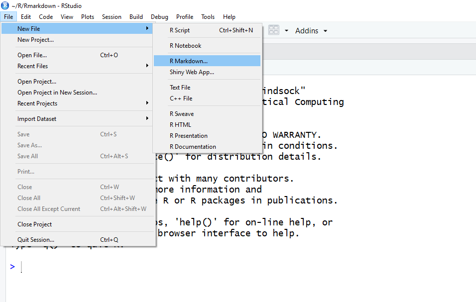
Start a new R markdown document in RStudio by clicking File > New File > R Markdown…

If this is the first time you have ever opened an R markdown file a dialog box will open up to tell you what packages need to be installed.

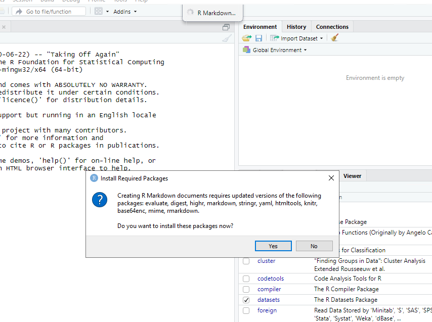
Click “Yes”. The packages will take a few seconds to install. You should see that each package was installed successfully in the dialog box.

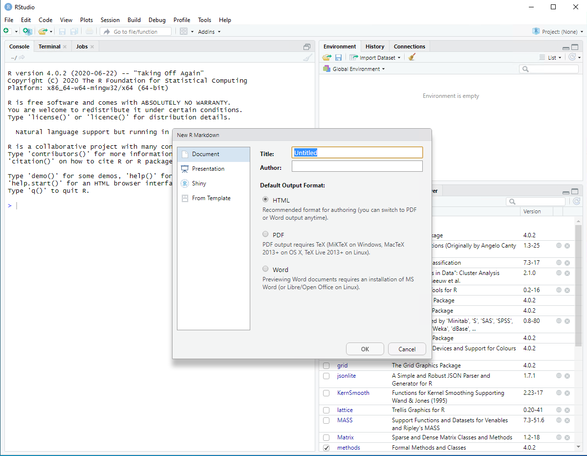
Once the package installs have completed, a dialog box will pop up and ask you to name the file and add an author name (may already know what your name is) The default output is HTML and as the wizard indicates, it is the best way to start and in your final version or later versions you have the option of changing to pdf or word document (among many other output formats! We’ll see this later).

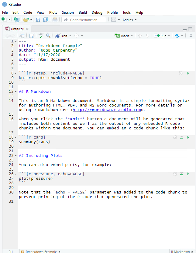
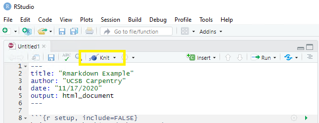
New R Markdown will always pop up with a generic template…

If you see this template you’re good to go.

Now we’ll get into how our R Markdown file & workflow is organized and then on to editing and styling!

R Markdown Workflow

R Markdown has four distinct steps in the workflow:

1. create a YAML header (optional)
2. write R Markdown-formatted text
3. add R code chunks for embedded analysis
4. render the document with Knitr
   
   

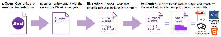
Let’s dig in to those more:

1. YAML header:

What is YAML anyway?

YAML, pronounced “Yeah-mul” stands for “YAML Ain’t Markup Language”. YAML is a human-readable data-serialization language which, as its name suggests, is not a markup language. YAML has no executable commands though it is compatible with all programming languages and virtually any application that deals with storing or transmiting data. YAML itself is made up of bits of many languages including Perl, MIME, C, & HTML. YAML is also a superset of JSON. When used as a stand-alone file the file ending is .yml or .yaml.

R Markdown’s default YAML header includes the following metadata surrounded by three dashes ---:

• title
• author
• date
• output

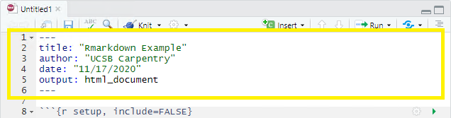
The first three are self-explanatory, but what’s the output? We saw this in the wizard for starting a new document, by default you are able to pick from pdf, html, and word document. Basically, this allows you to export your rmd file as a file type of your choice. There are other options for output and even more can be added by installing certain packages, but these are the three default options.

We’ll see other formatting options for YAML later on including how to add bibliography information, customize our output, and change the default settings of the knit function. Below is an example of how our YAML file will look at the end of this workshop.

---
title: "An Adapted Survey on Scientific Shared Resource Rigor and Reproducibility"
author: UCSB Carpentry
date: "December 16, 2020"
output:
  html_document:
    number_sections: true
bibliography: ../docs/bibliography.bibtex
csl: ../bin/apa-5th-edition.csl
knit: (function(inputFile, encoding) { 
      out_dir <- '../results';
      rmarkdown::render(inputFile,
                        encoding=encoding, 
                        output_file=file.path(dirname(inputFile), out_dir, 'Paper_Template_html.html')) })
---

2. Formatted text:

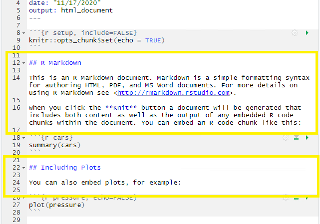
This one is simple, it’s literally just text narrative formatted by using markdown (more on markdown syntax later). Markdown-formatted text is one of the benefits added above and beyond the capabilities of a regular r script. Any text section will have the default white background in the rmd document. As you might know, in a regular R file, # starts a comment. In R markdown, plain text is just plain narrative text that appears in the document. In R scripts, plain text wants to be code. In R Markdown, you will need to enclose your code in special characters. Any symbols you do see that aren’t regular grammar components are for formatting, such as ##, ** **, and < >.

CHALLENGE 2.3 - Formatting with Symbols (optional)

In Rmd certain symbols are used to denote formatting that should happen to the text (after we “knit” or render). Before we knit, these symbols will show up seemingly “randomly” throughout the text and don’t contribute to the narrative in a logical way. In the generic Rmd document, there are three types of such symbols (##, **, <>) . Each symbol represents a different kind of formatting (think of your text formatting buttons you use in Word). Can you deduce from the surrounding text how these symbols format the surrounding text?

## R Markdown

This is an R Markdown document. Markdown is a simple formatting syntax for authoring HTML, PDF, and MS Word documents. For more details on using R Markdown see <http://rmarkdown.rstudio.com>.

When you click the **Knit** button a document will be generated that includes both content as well as the >output of any embedded R code chunks within the document. You can embed an R code chunk like this:

SOLUTION

## is a heading, ** is to bold enclosed text, and <> is for hyperlinks. Don’t worry about this too much right now! This is an example of R Markdown syntax for styling, we’ll dive into this next.

3. Code Chunks:

R code chunks appear highlighted in gray throughout the rmd document. They are surrounded by three tick marks on either side (```) with the starting three tick marks followed by curly brackets {}with some other code inside. The tick marks indicate the start of a code section and the bits found between the curly brackets {}indicate how R should read and display the code (more on this in the Knitr syntax episodes). These are the sections you add R code such as summary statistics, analysis, tables and plots. If you’ve already written an R script you can copy and paste your code between the few lines of required formatting to embed & run whichever piece you want at that particular spot in the document.

4. Rendering your Rmd document:

This is called “knitting”” and the button looks like a spool of yarn with a knitting needle. Clicking the knit button will compile the code, check for errors, and finally, output the type of file indicated in your yaml header. One nice thing about the knit button is that it saves the .Rmd document each time you run it. Your rmd document may not run and render as your indicated output if there are any errors in the document so it also functions somewhat as a code checker.

Try it yourself

We’re going to pause here and see what the R Markdown does when it’s rendered. We’ll just use the generic template, but when we’re working on our own project, knitting periodically while we’re editing allows us to catch errors early. We’ll continue rendering our rmd throughout the lesson to see what happens when we add our markdown and knitr syntax and to make sure we aren’t making any errors.

This is a little preview of what’s to come in the Knitr syntax episodes later on. Click the “knit” button

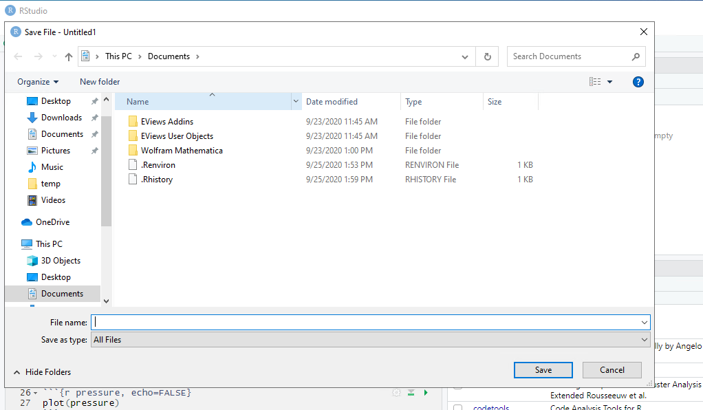
Before you can render your document, you’ll need to give it a file name and choose what folder you want to save it to. Choose rmd-workshop-paper.rmd as your file name and save the file to your code sub-folder.

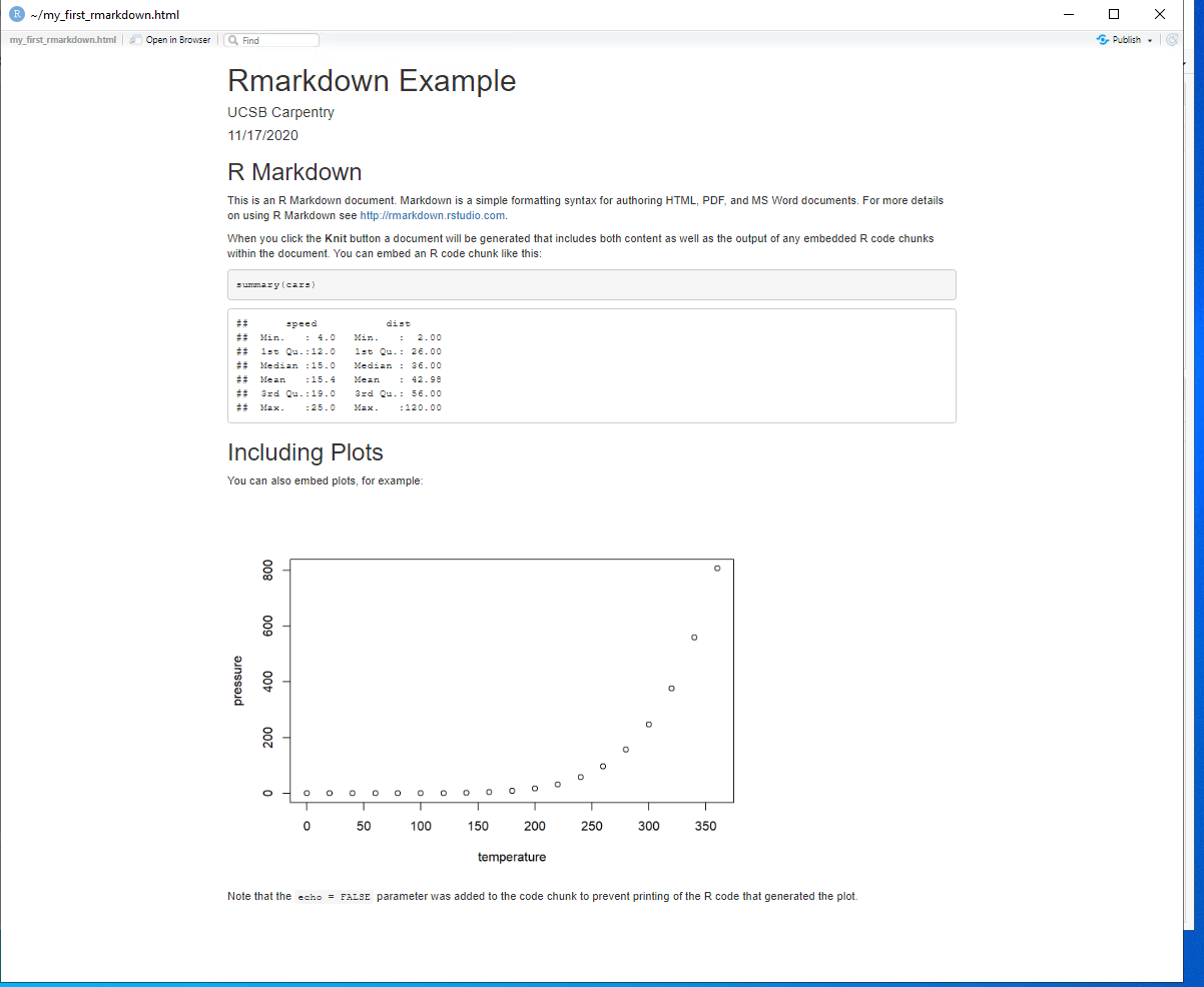
This is how our hmtl document will render after clicking the knit button and choosing a file name:

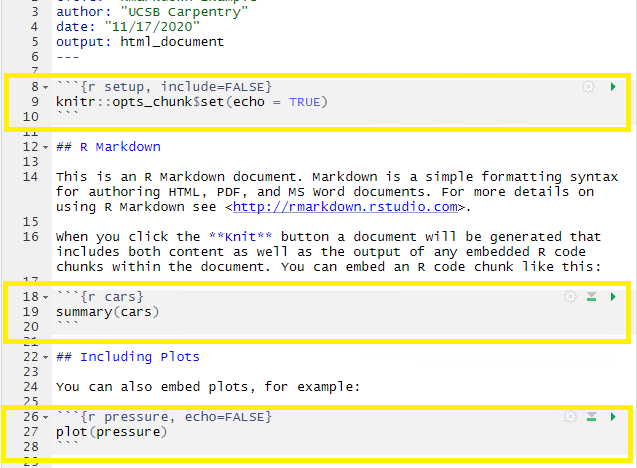
CHALLENGE 2.4 - echo=TRUE Function (optional)

Can you deduce what the echo=TRUE option stands for?

Solution

The echo=TRUE piece is knitr syntax that sets a global default for the whole paper. This piece of code specifically, echo=TRUE, tells the rmd document to display the R code that generates the plots & analysis when the rmd document is rendered by hitting the “knit” button. Don’t worry too much about this now, we’ll learn more about this syntax in the Knitr Syntax episodes.

Starting our paper

Ok, now let’s start on our own rmd document.

Do this on your own in your new rmd file:

1) Delete EVERYTHING except the yaml header

2) Edit the yaml header to add the title of the paper we’re working on and to add yourself as author.

---
title: "An Adapted Survey on Scientific Shared Resource Rigor and Reproducibility"
author: [Add Your Name Here]
date: "December 16, 2020"
output: html_document
---

3) Navigate to the docs folder and open paper_raw.txt. Copy all the text with either ctrl-a or cmd-a then ctrl-c or cmd-c and paste ctrl-v or cmd-v AFTER the yaml header in our rmd file.

...
output:
  html_document
---
INTRODUCTION
Reproducible research practices include rigorously controlled and documented experiments using validated reagents. These practices are integral to the scientific method, and they enable acquisition of reliable and actionable research results. However, the art and practice of science is affected by challenges 
...

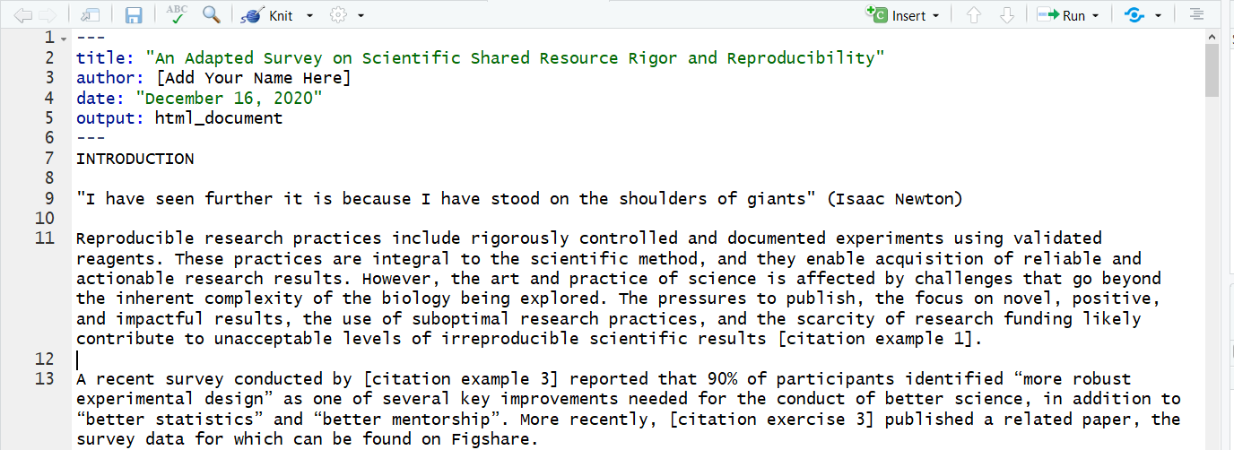
Your file should now look something like this:

Now we’ll be set for our next episode which is about adding Markdown syntax to style your text sections (white sections)- including headers, bold, italics, citations, footnotes, links, citations etc.

Key Points

• Starting a new Rmd File

• Anatomy of an Rmd File (YAML header, Text, Code chunks)

• How to knit an Rmd File to html