Introduction to R and RStudio
Overview
Teaching: 45 min
Exercises: 10 minQuestions
How to find your way around RStudio?
How to interact with R?
How to manage your environment?
How to install packages?
Objectives
Describe the purpose and use of each pane in the RStudio IDE
Locate buttons and options in the RStudio IDE
Define a variable
Assign data to a variable
Manage a workspace in an interactive R session
Use mathematical and comparison operators
Call functions
Manage packages
Motivation
Science is a multi-step process: once you’ve designed an experiment and collected data, the real fun begins! This lesson will teach you how to start this process using R and RStudio. We will begin with raw data, perform exploratory analyses, and learn how to plot results graphically. This example starts with a dataset from gapminder.org containing population information for many countries through time. Can you read the data into R? Can you plot the population for Senegal? Can you calculate the average income for countries on the continent of Asia? By the end of these lessons you will be able to do things like plot the populations for all of these countries in under a minute!
Before Starting The Workshop
Please ensure you have the latest version of R and RStudio installed on your machine. This is important, as some packages used in the workshop may not install correctly (or at all) if R is not up to date.
Introduction to RStudio
Welcome to the R portion of the Software Carpentry workshop.
Throughout this lesson, we’re going to teach you some of the fundamentals of the R language as well as some best practices for organizing code for scientific projects that will make your life easier.
We’ll be using RStudio: a free, open-source R Integrated Development Environment (IDE). It provides a built-in editor, works on all platforms (including on servers) and provides many advantages such as integration with version control and project management.
Basic layout
When you first open RStudio, you will be greeted by three panels:
- The interactive R console/Terminal (entire left)
- Environment/History/Connections (tabbed in upper right)
- Files/Plots/Packages/Help/Viewer (tabbed in lower right)
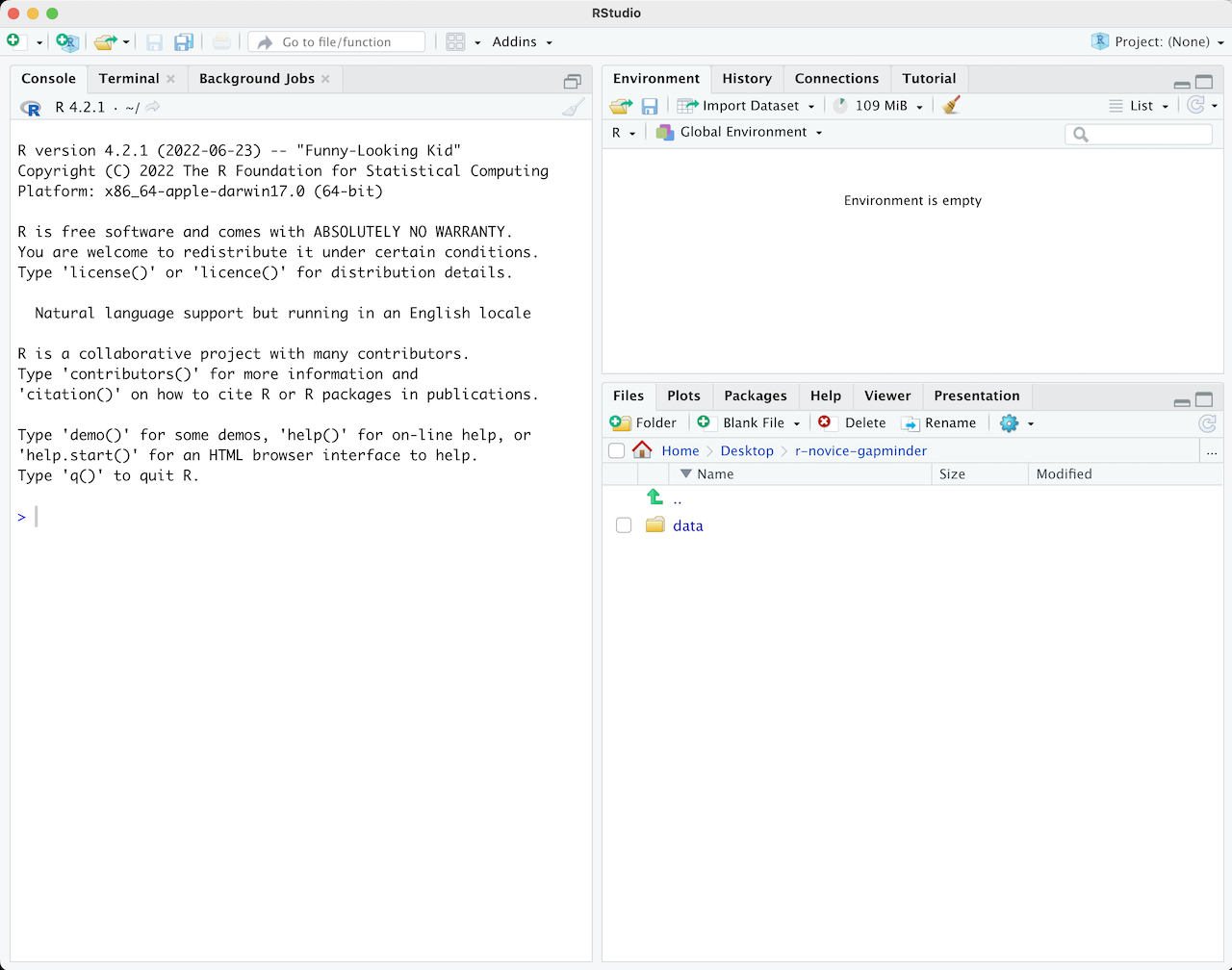
Once you open files, such as R scripts, an editor panel will also open in the top left.
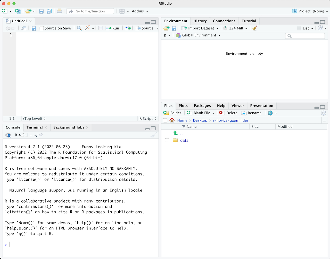
R scripts
Any commands that you write in the R console can be saved in to a file to be re-run again. Files containg R code to be ran in this way are called R scripts. R scripts have
.Rat the end of their names to let you know what they are.
Workflow within RStudio
There are two main ways one can work within RStudio:
- Test and play within the interactive R console then copy code into
a .R file to run later.
- This works well when doing small tests and initially starting off.
- It quickly becomes laborious
- Start writing in a .R file and use RStudio’s short cut keys for the Run command
to push the current line, selected lines or modified lines to the
interactive R console.
- This is a great way to start; all your code is saved for later
- You will be able to run the file you create from within RStudio
or using R’s
source()function.
Tip: Running segments of your code
RStudio offers you great flexibility in running code from within the editor window. There are buttons, menu choices, and keyboard shortcuts. To run the current line, you can
- click on the
Runbutton above the editor panel, or- select “Run Lines” from the “Code” menu, or
- hit Ctrl+Return in Windows or Linux or ⌘+Return on OS X. (This shortcut can also be seen by hovering the mouse over the button). To run a block of code, select it and then
Run. If you have modified a line of code within a block of code you have just run, there is no need to reselect the section andRun, you can use the next button along,Re-run the previous region. This will run the previous code block including the modifications you have made.
Introduction to R
Much of your time in R will be spent in the R interactive
console. This is where you will run all of your code, and can be a
useful environment to try out ideas before adding them to an R script
file. This console in RStudio is the same as the one you would get if
you typed in R in your command-line environment.
The first thing you will see in the R interactive session is a bunch of information, followed by a “>” and a blinking cursor. In many ways this is similar to the shell environment you learned about during the shell lessons: it operates on the same idea of a “Read, evaluate, print loop”: you type in commands, R tries to execute them, and then returns a result.
Using R as a calculator
The simplest thing you could do with R is to do arithmetic:
1 + 100
[1] 101
And R will print out the answer, with a preceding “[1]”. Don’t worry about this for now, we’ll explain that later. For now think of it as indicating output.
If you type in an incomplete command, R will wait for you to
complete it. If you are familiar with Unix Shell’s bash, you may recognize this
behavior from bash.
> 1 +
+
Any time you hit return and the R session shows a “+” instead of a “>”, it means it’s waiting for you to complete the command. If you want to cancel a command you can hit Esc and RStudio will give you back the “>” prompt.
Tip: Canceling commands
If you’re using R from the command line instead of from within RStudio, you need to use Ctrl+C instead of Esc to cancel the command. This applies to Mac users as well!
Canceling a command isn’t only useful for killing incomplete commands: you can also use it to tell R to stop running code (for example if it’s taking much longer than you expect), or to get rid of the code you’re currently writing.
When using R as a calculator, the order of operations is the same as you would have learned back in school.
From highest to lowest precedence:
- Parentheses:
(,) - Exponents:
^or** - Multiply:
* - Divide:
/ - Add:
+ - Subtract:
-
3 + 5 * 2
[1] 13
Use parentheses to group operations in order to force the order of evaluation if it differs from the default, or to make clear what you intend.
(3 + 5) * 2
[1] 16
This can get unwieldy when not needed, but clarifies your intentions. Remember that others may later read your code.
(3 + (5 * (2 ^ 2))) # hard to read
3 + 5 * 2 ^ 2       # clear, if you remember the rules
3 + 5 * (2 ^ 2)     # if you forget some rules, this might help
The text after each line of code is called a
“comment”. Anything that follows after the hash (or octothorpe) symbol
# is ignored by R when it executes code.
Really small or large numbers get a scientific notation:
2/10000
[1] 2e-04
Which is shorthand for “multiplied by 10^XX”. So 2e-4
is shorthand for 2 * 10^(-4).
You can write numbers in scientific notation too:
5e3 # Note the lack of minus here
[1] 5000
Mathematical functions
R has many built in mathematical functions. To call a function, we can type its name, followed by open and closing parentheses. Functions take arguments as inputs, anything we type inside the parentheses of a function is considered an argument. Depending on the function, the number of arguments can vary from none to multiple. For example:
getwd() #returns an absolute filepath
doesn’t require an argument, whereas for the next set of mathematical functions we will need to supply the function a value in order to compute the result.
sin(1) # trigonometry functions
[1] 0.841471
log(1) # natural logarithm
[1] 0
log10(10) # base-10 logarithm
[1] 1
exp(0.5) # e^(1/2)
[1] 1.648721
Don’t worry about trying to remember every function in R. You can look them up on Google, or if you can remember the start of the function’s name, use the tab completion in RStudio.
This is one advantage that RStudio has over R on its own, it has auto-completion abilities that allow you to more easily look up functions, their arguments, and the values that they take.
Typing a ? before the name of a command will open the help page
for that command. When using RStudio, this will open the ‘Help’ pane;
if using R in the terminal, the help page will open in your browser.
The help page will include a detailed description of the command and
how it works. Scrolling to the bottom of the help page will usually
show a collection of code examples which illustrate command usage.
We’ll go through an example later.
Comparing things
We can also do comparisons in R:
1 == 1 # equality (note two equals signs, read as "is equal to")
[1] TRUE
1 != 2 # inequality (read as "is not equal to")
[1] TRUE
1 < 2 # less than
[1] TRUE
1 <= 1 # less than or equal to
[1] TRUE
1 > 0 # greater than
[1] TRUE
1 >= -9 # greater than or equal to
[1] TRUE
Tip: Comparing Numbers
A word of warning about comparing numbers: you should never use
==to compare two numbers unless they are integers (a data type which can specifically represent only whole numbers).Computers may only represent decimal numbers with a certain degree of precision, so two numbers which look the same when printed out by R, may actually have different underlying representations and therefore be different by a small margin of error (called Machine numeric tolerance).
Instead you should use the
all.equalfunction.Further reading: http://floating-point-gui.de/
Variables and assignment
We can store values in variables using the assignment operator <-, like this:
x <- 1/40
Notice that assignment does not print a value. Instead, we stored it for later
in something called a variable. x now contains the value 0.025:
x
[1] 0.025
More precisely, the stored value is a decimal approximation of this fraction called a floating point number.
Look for the Environment tab in the top right panel of RStudio, and you will see that x and its value
have appeared. Our variable x can be used in place of a number in any calculation that expects a number:
log(x)
[1] -3.688879
Notice also that variables can be reassigned:
x <- 100
x used to contain the value 0.025 and now it has the value 100.
Assignment values can contain the variable being assigned to:
x <- x + 1 #notice how RStudio updates its description of x on the top right tab
y <- x * 2
The right hand side of the assignment can be any valid R expression. The right hand side is fully evaluated before the assignment occurs.
Variable names can contain letters, numbers, underscores and periods but no spaces. They must start with a letter or a period followed by a letter (they cannot start with a number nor an underscore). Variables beginning with a period are hidden variables. Different people use different conventions for long variable names, these include
- periods.between.words
- underscores_between_words
- camelCaseToSeparateWords
What you use is up to you, but be consistent.
It is also possible to use the = operator for assignment:
x = 1/40
But this is much less common among R users. The most important thing is to
be consistent with the operator you use. There are occasionally places
where it is less confusing to use <- than =, and it is the most common
symbol used in the community. So the recommendation is to use <-.
Challenge 1
Which of the following are valid R variable names?
min_height
max.height
_age
.mass
MaxLength
min-length
2widths
celsius2kelvin
Solution to challenge 1
The following can be used as R variables:
min_height
max.height
MaxLength
celsius2kelvin
The following creates a hidden variable:
.massThe following will not be able to be used to create a variable
_age
min-length
2widths
Vectorization
One final thing to be aware of is that R is vectorized, meaning that variables and functions can have vectors as values. In contrast to physics and mathematics, a vector in R describes a set of values in a certain order of the same data type. For example
1:5
[1] 1 2 3 4 5
2^(1:5)
[1] 2 4 8 16 32
x <- 1:5
2^x
[1] 2 4 8 16 32
This is incredibly powerful; we will discuss this further in an upcoming lesson.
Managing your environment
There are a few useful commands you can use to interact with the R session.
ls will list all of the variables and functions stored in the global environment
(your working R session):
ls()
[1] "args" "dest_md" "op" "src_rmd" "x" "y"
Tip: hidden objects
Like in the shell,
lswill hide any variables or functions starting with a “.” by default. To list all objects, typels(all.names=TRUE)instead
Note here that we didn’t give any arguments to ls, but we still
needed to give the parentheses to tell R to call the function.
If we type ls by itself, R prints a bunch of code instead of a listing of objects.
ls
function (name, pos = -1L, envir = as.environment(pos), all.names = FALSE,
    pattern, sorted = TRUE)
{
    if (!missing(name)) {
        pos <- tryCatch(name, error = function(e) e)
        if (inherits(pos, "error")) {
            name <- substitute(name)
            if (!is.character(name))
                name <- deparse(name)
            warning(gettextf("%s converted to character string",
                sQuote(name)), domain = NA)
            pos <- name
        }
    }
    all.names <- .Internal(ls(envir, all.names, sorted))
    if (!missing(pattern)) {
        if ((ll <- length(grep("[", pattern, fixed = TRUE))) &&
            ll != length(grep("]", pattern, fixed = TRUE))) {
            if (pattern == "[") {
                pattern <- "\\["
                warning("replaced regular expression pattern '[' by  '\\\\['")
            }
            else if (length(grep("[^\\\\]\\[<-", pattern))) {
                pattern <- sub("\\[<-", "\\\\\\[<-", pattern)
                warning("replaced '[<-' by '\\\\[<-' in regular expression pattern")
            }
        }
        grep(pattern, all.names, value = TRUE)
    }
    else all.names
}
<bytecode: 0x5644cbc309c8>
<environment: namespace:base>
What’s going on here?
Like everything in R, ls is the name of an object, and entering the name of
an object by itself prints the contents of the object. The object x that we
created earlier contains 1, 2, 3, 4, 5:
x
[1] 1 2 3 4 5
The object ls contains the R code that makes the ls function work! We’ll talk
more about how functions work and start writing our own later.
You can use rm to delete objects you no longer need:
rm(x)
If you have lots of things in your environment and want to delete all of them,
you can pass the results of ls to the rm function:
rm(list = ls())
In this case we’ve combined the two. Like the order of operations, anything inside the innermost parentheses is evaluated first, and so on.
In this case we’ve specified that the results of ls should be used for the
list argument in rm. When assigning values to arguments by name, you must
use the = operator!!
If instead we use <-, there will be unintended side effects, or you may get an error message:
rm(list <- ls())
Error in rm(list <- ls()): ... must contain names or character strings
Tip: Warnings vs. Errors
Pay attention when R does something unexpected! Errors, like above, are thrown when R cannot proceed with a calculation. Warnings on the other hand usually mean that the function has run, but it probably hasn’t worked as expected.
In both cases, the message that R prints out usually give you clues how to fix a problem.
R Packages
It is possible to add functions to R by writing a package, or by obtaining a package written by someone else. As of this writing, there are over 10,000 packages available on CRAN (the comprehensive R archive network). R and RStudio have functionality for managing packages:
- You can see what packages are installed by typing
installed.packages() - You can install packages by typing
install.packages("packagename"), wherepackagenameis the package name, in quotes. - You can update installed packages by typing
update.packages() - You can remove a package with
remove.packages("packagename") - You can make a package available for use with
library(packagename)
Packages can also be viewed, loaded, and detached in the Packages tab of the lower right panel in RStudio. Clicking on this tab will display all of the installed packages with a checkbox next to them. If the box next to a package name is checked, the package is loaded and if it is empty, the package is not loaded. Click an empty box to load that package and click a checked box to detach that package.
Packages can be installed and updated from the Package tab with the Install and Update buttons at the top of the tab.
Challenge 2
What will be the value of each variable after each statement in the following program?
mass <- 47.5
age <- 122
mass <- mass * 2.3
age <- age - 20
Solution to challenge 2
mass <- 47.5This will give a value of 47.5 for the variable mass
age <- 122This will give a value of 122 for the variable age
mass <- mass * 2.3This will multiply the existing value of 47.5 by 2.3 to give a new value of 109.25 to the variable mass.
age <- age - 20This will subtract 20 from the existing value of 122 to give a new value of 102 to the variable age.
Challenge 3
Run the code from the previous challenge, and write a command to compare mass to age. Is mass larger than age?
Solution to challenge 3
One way of answering this question in R is to use the
>to set up the following:mass > age[1] TRUEThis should yield a boolean value of TRUE since 109.25 is greater than 102.
Challenge 4
Clean up your working environment by deleting the mass and age variables.
Solution to challenge 4
We can use the
rmcommand to accomplish this taskrm(age, mass)
Challenge 5
Install the following packages:
ggplot2,plyr,gapminderSolution to challenge 5
We can use the
install.packages()command to install the required packages.install.packages("ggplot2") install.packages("plyr") install.packages("gapminder")An alternate solution, to install multiple packages with a single
install.packages()command is:install.packages(c("ggplot2", "plyr", "gapminder"))
Key Points
Use RStudio to write and run R programs.
R has the usual arithmetic operators and mathematical functions.
Use
<-to assign values to variables.Use
ls()to list the variables in a program.Use
rm()to delete objects in a program.Use
install.packages()to install packages (libraries).
Project Management With RStudio
Overview
Teaching: 20 min
Exercises: 10 minQuestions
How can I manage my projects in R?
Objectives
Create self-contained projects in RStudio
Introduction
The scientific process is naturally incremental, and many projects start life as random notes, some code, then a manuscript, and eventually everything is a bit mixed together.
Managing your projects in a reproducible fashion doesn't just make your science reproducible, it makes your life easier.
— Vince Buffalo (@vsbuffalo) April 15, 2013
Most people tend to organize their projects like this:
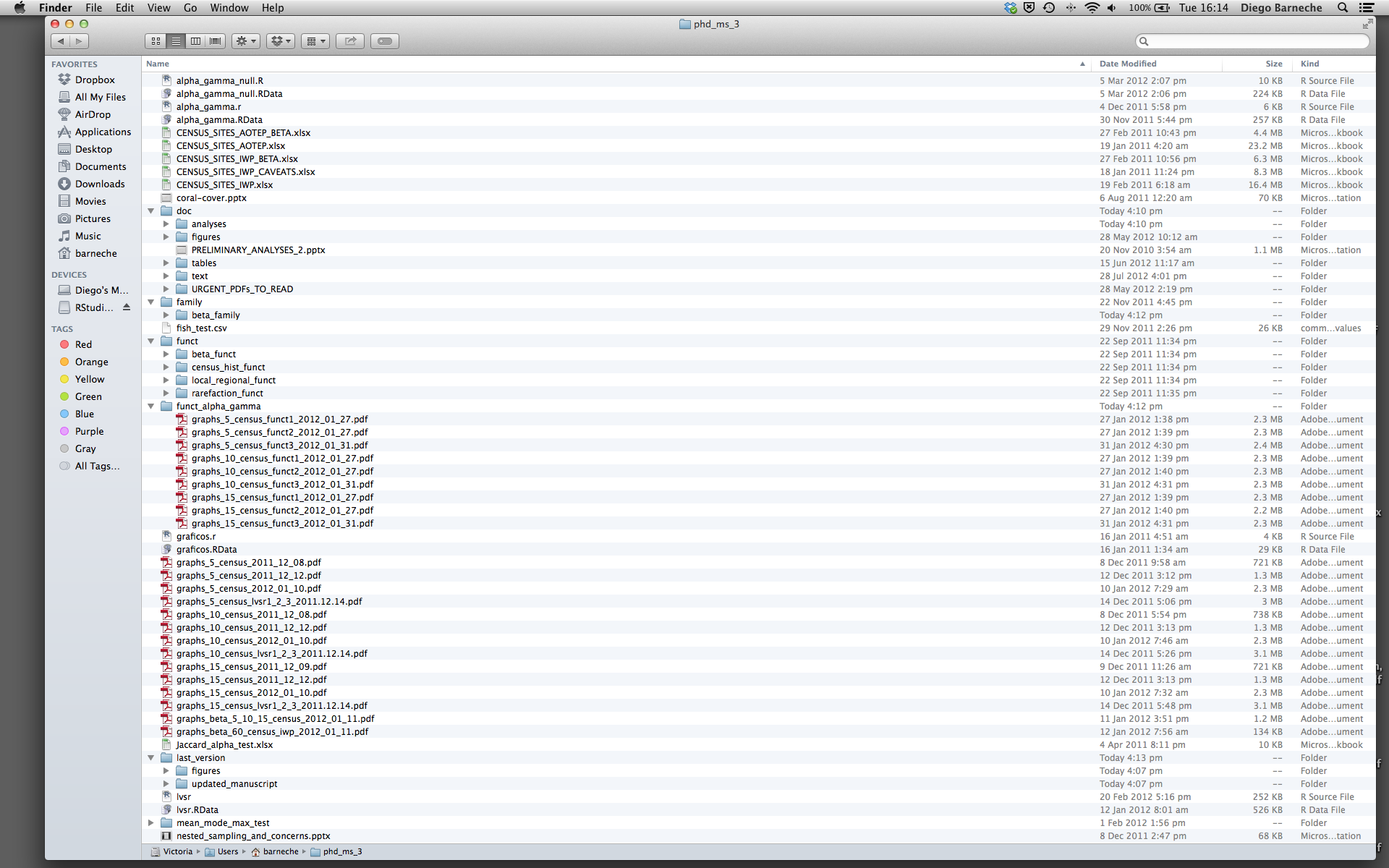
There are many reasons why we should ALWAYS avoid this:
- It is really hard to tell which version of your data is the original and which is the modified;
- It gets really messy because it mixes files with various extensions together;
- It probably takes you a lot of time to actually find things, and relate the correct figures to the exact code that has been used to generate it;
A good project layout will ultimately make your life easier:
- It will help ensure the integrity of your data;
- It makes it simpler to share your code with someone else (a lab-mate, collaborator, or supervisor);
- It allows you to easily upload your code with your manuscript submission;
- It makes it easier to pick the project back up after a break.
A possible solution
Fortunately, there are tools and packages which can help you manage your work effectively.
One of the most powerful and useful aspects of RStudio is its project management functionality. We’ll be using this today to create a self-contained, reproducible project.
Challenge 1: Creating a self-contained project
We’re going to create a new project in RStudio:
- Click the “File” menu button, then “New Project”.
- Click “New Directory”.
- Click “New Project”.
- Type in the name of the directory to store your project, e.g. “my_project”.
- If available, select the checkbox for “Create a git repository.”
- Click the “Create Project” button.
The simplest way to open an RStudio project once it has been created is to click
through your file system to get to the directory where it was saved and double
click on the .Rproj file. This will open RStudio and start your R session in the
same directory as the .Rproj file. All your data, plots and scripts will now be
relative to the project directory. RStudio projects have the added benefit of
allowing you to open multiple projects at the same time each open to its own
project directory. This allows you to keep multiple projects open without them
interfering with each other.
Challenge 2: Opening an RStudio project through the file system
- Exit RStudio.
- Navigate to the directory where you created a project in Challenge 1.
- Double click on the
.Rprojfile in that directory.
Best practices for project organization
Although there is no “best” way to lay out a project, there are some general principles to adhere to that will make project management easier:
Treat data as read only
This is probably the most important goal of setting up a project. Data is typically time consuming and/or expensive to collect. Working with them interactively (e.g., in Excel) where they can be modified means you are never sure of where the data came from, or how it has been modified since collection. It is therefore a good idea to treat your data as “read-only”.
Data Cleaning
In many cases your data will be “dirty”: it will need significant preprocessing to get into a format R (or any other programming language) will find useful. This task is sometimes called “data munging”. Storing these scripts in a separate folder, and creating a second “read-only” data folder to hold the “cleaned” data sets can prevent confusion between the two sets.
Treat generated output as disposable
Anything generated by your scripts should be treated as disposable: it should all be able to be regenerated from your scripts.
There are lots of different ways to manage this output. Having an output folder with different sub-directories for each separate analysis makes it easier later. Since many analyses are exploratory and don’t end up being used in the final project, and some of the analyses get shared between projects.
Tip: Good Enough Practices for Scientific Computing
Good Enough Practices for Scientific Computing gives the following recommendations for project organization:
- Put each project in its own directory, which is named after the project.
- Put text documents associated with the project in the
docdirectory.- Put raw data and metadata in the
datadirectory, and files generated during cleanup and analysis in aresultsdirectory.- Put source for the project’s scripts and programs in the
srcdirectory, and programs brought in from elsewhere or compiled locally in thebindirectory.- Name all files to reflect their content or function.
Separate function definition and application
One of the more effective ways to work with R is to start by writing the code you want to run directly in a .R script, and then running the selected lines (either using the keyboard shortcuts in RStudio or clicking the “Run” button) in the interactive R console.
When your project is in its early stages, the initial .R script file usually contains many lines of directly executed code. As it matures, reusable chunks get pulled into their own functions. It’s a good idea to separate these functions into two separate folders; one to store useful functions that you’ll reuse across analyses and projects, and one to store the analysis scripts.
Save the data in the data directory
Now we have a good directory structure we will now place/save the data file in the data/ directory.
Challenge 3
Download the gapminder data from here.
- Download the file (right mouse click on the link above -> “Save link as” / “Save file as”, or click on the link and after the page loads, press Ctrl+S or choose File -> “Save page as”)
- Make sure it’s saved under the name
gapminder_data.csv- Save the file in the
data/folder within your project.We will load and inspect these data later.
Challenge 4
It is useful to get some general idea about the dataset, directly from the command line, before loading it into R. Understanding the dataset better will come in handy when making decisions on how to load it in R. Use the command-line shell to answer the following questions:
- What is the size of the file?
- How many rows of data does it contain?
- What kinds of values are stored in this file?
Solution to Challenge 4
By running these commands in the shell:
ls -lh data/gapminder_data.csv-rw-r--r-- 1 runner docker 80K Nov 7 04:15 data/gapminder_data.csvThe file size is 80K.
wc -l data/gapminder_data.csv1705 data/gapminder_data.csvThere are 1705 lines. The data looks like:
head data/gapminder_data.csvcountry,year,pop,continent,lifeExp,gdpPercap Afghanistan,1952,8425333,Asia,28.801,779.4453145 Afghanistan,1957,9240934,Asia,30.332,820.8530296 Afghanistan,1962,10267083,Asia,31.997,853.10071 Afghanistan,1967,11537966,Asia,34.02,836.1971382 Afghanistan,1972,13079460,Asia,36.088,739.9811058 Afghanistan,1977,14880372,Asia,38.438,786.11336 Afghanistan,1982,12881816,Asia,39.854,978.0114388 Afghanistan,1987,13867957,Asia,40.822,852.3959448 Afghanistan,1992,16317921,Asia,41.674,649.3413952
Tip: command line in RStudio
The Terminal tab in the console pane provides a convenient place directly within RStudio to interact directly with the command line.
Working directory
Knowing R’s current working directory is important because when you need to access other files (for example, to import a data file), R will look for them relative to the current working directory.
Each time you create a new RStudio Project, it will create a new directory for that project. When you open an existing .Rproj file, it will open that project and set R’s working directory to the folder that file is in.
Challenge 5
You can check the current working directory with the
getwd()command, or by using the menus in RStudio.
- In the console, type
getwd()(“wd” is short for “working directory”) and hit Enter.- In the Files pane, double click on the
datafolder to open it (or navigate to any other folder you wish). To get the Files pane back to the current working directory, click “More” and then select “Go To Working Directory”.You can change the working directory with
setwd(), or by using RStudio menus.
- In the console, type
setwd("data")and hit Enter. Typegetwd()and hit Enter to see the new working directory.- In the menus at the top of the RStudio window, click the “Session” menu button, and then select “Set Working Directory” and then “Choose Directory”.
- In the windows navigator that opens, navigate back to the project directory, and click “Open”. Note that a
setwdcommand will automatically appear in the console.
Tip: File does not exist errors
When you’re attempting to reference a file in your R code and you’re getting errors saying the file doesn’t exist, it’s a good idea to check your working directory. You need to either provide an absolute path to the file, or you need to make sure the file is saved in the working directory (or a subfolder of the working directory) and provide a relative path.
Version Control
It is important to use version control with projects. Go here for a good lesson which describes using Git with RStudio.
Key Points
Use RStudio to create and manage projects with consistent layout.
Treat raw data as read-only.
Treat generated output as disposable.
Separate function definition and application.
Seeking Help
Overview
Teaching: 10 min
Exercises: 10 minQuestions
How can I get help in R?
Objectives
To be able to read R help files for functions and special operators.
To be able to use CRAN task views to identify packages to solve a problem.
To be able to seek help from your peers.
Reading Help Files
R, and every package, provide help files for functions. The general syntax to search for help on any function, “function_name”, from a specific function that is in a package loaded into your namespace (your interactive R session) is:
?function_name
help(function_name)
For example take a look at the help file for write.table(), we will be using a similar function in an upcoming episode.
?write.table()
This will load up a help page in RStudio (or as plain text in R itself).
Each help page is broken down into sections:
- Description: An extended description of what the function does.
- Usage: The arguments of the function and their default values (which can be changed).
- Arguments: An explanation of the data each argument is expecting.
- Details: Any important details to be aware of.
- Value: The data the function returns.
- See Also: Any related functions you might find useful.
- Examples: Some examples for how to use the function.
Different functions might have different sections, but these are the main ones you should be aware of.
Notice how related functions might call for the same help file:
?write.table()
?write.csv()
This is because these functions have very similar applicability and often share the same arguments as inputs to the function, so package authors often choose to document them together in a single help file.
Tip: Running Examples
From within the function help page, you can highlight code in the Examples and hit Ctrl+Return to run it in RStudio console. This gives you a quick way to get a feel for how a function works.
Tip: Reading Help Files
One of the most daunting aspects of R is the large number of functions available. It would be prohibitive, if not impossible to remember the correct usage for every function you use. Luckily, using the help files means you don’t have to remember that!
Special Operators
To seek help on special operators, use quotes or backticks:
?"<-"
?`<-`
Getting Help with Packages
Many packages come with “vignettes”: tutorials and extended example documentation.
Without any arguments, vignette() will list all vignettes for all installed packages;
vignette(package="package-name") will list all available vignettes for
package-name, and vignette("vignette-name") will open the specified vignette.
If a package doesn’t have any vignettes, you can usually find help by typing
help("package-name").
RStudio also has a set of excellent cheatsheets for many packages.
When You Remember Part of the Function Name
If you’re not sure what package a function is in or how it’s specifically spelled, you can do a fuzzy search:
??function_name
A fuzzy search is when you search for an approximate string match. For example, you may remember that the function to set your working directory includes “set” in its name. You can do a fuzzy search to help you identify the function:
??set
When You Have No Idea Where to Begin
If you don’t know what function or package you need to use CRAN Task Views is a specially maintained list of packages grouped into fields. This can be a good starting point.
When Your Code Doesn’t Work: Seeking Help from Your Peers
If you’re having trouble using a function, 9 times out of 10,
the answers you seek have already been answered on
Stack Overflow. You can search using
the [r] tag. Please make sure to see their page on
how to ask a good question.
If you can’t find the answer, there are a few useful functions to help you ask your peers:
?dput
Will dump the data you’re working with into a format that can be copied and pasted by others into their own R session.
sessionInfo()
R version 4.2.1 (2022-06-23)
Platform: x86_64-pc-linux-gnu (64-bit)
Running under: Ubuntu 20.04.5 LTS

Matrix products: default
BLAS:   /usr/lib/x86_64-linux-gnu/blas/libblas.so.3.9.0
LAPACK: /usr/lib/x86_64-linux-gnu/lapack/liblapack.so.3.9.0

locale:
 [1] LC_CTYPE=C.UTF-8       LC_NUMERIC=C           LC_TIME=C.UTF-8
 [4] LC_COLLATE=C.UTF-8     LC_MONETARY=C.UTF-8    LC_MESSAGES=C.UTF-8
 [7] LC_PAPER=C.UTF-8       LC_NAME=C              LC_ADDRESS=C
[10] LC_TELEPHONE=C         LC_MEASUREMENT=C.UTF-8 LC_IDENTIFICATION=C

attached base packages:
[1] stats     graphics  grDevices utils     datasets  methods   base

other attached packages:
[1] knitr_1.40

loaded via a namespace (and not attached):
[1] compiler_4.2.1 magrittr_2.0.3 tools_4.2.1    stringi_1.7.8  stringr_1.4.1
[6] xfun_0.34      evaluate_0.17
Will print out your current version of R, as well as any packages you have loaded. This can be useful for others to help reproduce and debug your issue.
Challenge 1
Look at the help page for the
cfunction. What kind of vector do you expect will be created if you evaluate the following:c(1, 2, 3) c('d', 'e', 'f') c(1, 2, 'f')Solution to Challenge 1
The
c()function creates a vector, in which all elements are of the same type. In the first case, the elements are numeric, in the second, they are characters, and in the third they are also characters: the numeric values are “coerced” to be characters.
Challenge 2
Look at the help for the
pastefunction. You will need to use it later. What’s the difference between thesepandcollapsearguments?Solution to Challenge 2
To look at the help for the
paste()function, use:help("paste") ?pasteThe difference between
sepandcollapseis a little tricky. Thepastefunction accepts any number of arguments, each of which can be a vector of any length. Thesepargument specifies the string used between concatenated terms — by default, a space. The result is a vector as long as the longest argument supplied topaste. In contrast,collapsespecifies that after concatenation the elements are collapsed together using the given separator, the result being a single string.It is important to call the arguments explicitly by typing out the argument name e.g
sep = ","so the function understands to use the “,” as a separator and not a term to concatenate. e.g.paste(c("a","b"), "c")[1] "a c" "b c"paste(c("a","b"), "c", ",")[1] "a c ," "b c ,"paste(c("a","b"), "c", sep = ",")[1] "a,c" "b,c"paste(c("a","b"), "c", collapse = "|")[1] "a c|b c"paste(c("a","b"), "c", sep = ",", collapse = "|")[1] "a,c|b,c"(For more information, scroll to the bottom of the
?pastehelp page and look at the examples, or tryexample('paste').)
Challenge 3
Use help to find a function (and its associated parameters) that you could use to load data from a tabular file in which columns are delimited with “\t” (tab) and the decimal point is a “.” (period). This check for decimal separator is important, especially if you are working with international colleagues, because different countries have different conventions for the decimal point (i.e. comma vs period). Hint: use
??"read table"to look up functions related to reading in tabular data.Solution to Challenge 3
The standard R function for reading tab-delimited files with a period decimal separator is read.delim(). You can also do this with
read.table(file, sep="\t")(the period is the default decimal separator forread.table()), although you may have to change thecomment.charargument as well if your data file contains hash (#) characters.
Other Resources
Key Points
Use
help()to get online help in R.
Data Structures
Overview
Teaching: 40 min
Exercises: 15 minQuestions
How can I read data in R?
What are the basic data types in R?
How do I represent categorical information in R?
Objectives
To be able to identify the 5 main data types.
To begin exploring data frames, and understand how they are related to vectors, factors and lists.
To be able to ask questions from R about the type, class, and structure of an object.
One of R’s most powerful features is its ability to deal with tabular data -
such as you may already have in a spreadsheet or a CSV file. Let’s start by
making a toy dataset in your output_data/ directory, called feline-data.csv:
cats <- data.frame(coat = c("calico", "black", "tabby"),
                    weight = c(2.1, 5.0, 3.2),
                    likes_string = c(1, 0, 1))
We can now save cats as a CSV file. It is good practice to call the argument
names explicitly so the function knows what default values you are changing. Here we
are setting row.names = FALSE. Recall you can use ?write.csv to pull
up the help file to check out the argument names and their default values.
write.csv(x = cats, file = "data/feline-data.csv", row.names = FALSE)
The contents of the new file, feline-data.csv:
coat,weight,likes_string
calico,2.1,1
black,5.0,0
tabby,3.2,1
Tip: Editing Text files in R
Alternatively, you can create
output_data/feline-data.csvusing a text editor (Nano), or within RStudio with the File -> New File -> Text File menu item.
We can load this into R via the following:
cats <- read.csv(file = "output_data/feline-data.csv", stringsAsFactors = TRUE)
cats
    coat weight likes_string
1 calico    2.1            1
2  black    5.0            0
3  tabby    3.2            1
The read.table function is used for reading in tabular data stored in a text
file where the columns of data are separated by punctuation characters such as
CSV files (csv = comma-separated values). Tabs and commas are the most common
punctuation characters used to separate or delimit data points in csv files.
For convenience R provides 2 other versions of read.table. These are: read.csv
for files where the data are separated with commas and read.delim for files
where the data are separated with tabs. Of these three functions read.csv is
the most commonly used. If needed it is possible to override the default
delimiting punctuation marks for both read.csv and read.delim.
We can begin exploring our dataset right away, pulling out columns by specifying
them using the $ operator:
cats$weight
[1] 2.1 5.0 3.2
cats$coat
[1] calico black  tabby
Levels: black calico tabby
We can do other operations on the columns:
## Say we discovered that the scale weighs two Kg light:
cats$weight + 2
[1] 4.1 7.0 5.2
paste("My cat is", cats$coat)
[1] "My cat is calico" "My cat is black" "My cat is tabby"
But what about
cats$weight + cats$coat
Warning in Ops.factor(cats$weight, cats$coat): '+' not meaningful for factors
[1] NA NA NA
Understanding what happened here is key to successfully analyzing data in R.
Data Types
If you guessed that the last command will return an error because 2.1 plus
"black" is nonsense, you’re right - and you already have some intuition for an
important concept in programming called data types. We can ask what type of
data something is:
typeof(cats$weight)
[1] "double"
There are 5 main types: double, integer, complex, logical and character.
typeof(3.14)
[1] "double"
typeof(1L) # The L suffix forces the number to be an integer, since by default R uses float numbers
[1] "integer"
typeof(1+1i)
[1] "complex"
typeof(TRUE)
[1] "logical"
typeof('banana')
[1] "character"
No matter how complicated our analyses become, all data in R is interpreted as one of these basic data types. This strictness has some really important consequences.
A user has added details of another cat. This information is in the file
data/feline-data_v2.csv.
file.show("data/feline-data_v2.csv")
coat,weight,likes_string
calico,2.1,1
black,5.0,0
tabby,3.2,1
tabby,2.3 or 2.4,1
Load the new cats data like before, and check what type of data we find in the
weight column:
cats <- read.csv(file="data/feline-data_v2.csv", stringsAsFactors = TRUE)
typeof(cats$weight)
[1] "integer"
Oh no, our weights aren’t the double type anymore! If we try to do the same math we did on them before, we run into trouble:
cats$weight + 2
Warning in Ops.factor(cats$weight, 2): '+' not meaningful for factors
[1] NA NA NA NA
What happened?
The cats data we are working with is something called a data frame. Data frames
are one of the most common and versatile types of data structures we will work with in R.
In this example, the columns that make up the data frame cannot be composed of different data types.
In this case, R does not read everything in the data frame as a double, therefore the entire
column data type changes to something that is suitable for everything in the column.
When R reads a csv file, it reads it in as a data frame. Thus, when we loaded the cats
csv file, it is stored as a data frame. We can check this by using the function class().
class(cats)
[1] "data.frame"
Data frames are composed of rows and columns, where each column has the same number of rows. Different columns in a data frame can be made up of different data types (this is what makes them so versatile), but everything in a given column needs to be the same type (e.g., vector, factor, or list).
Let’s explore more about different data structures and how they behave. For now, let’s remove that extra line from our cats data and reload it, while we investigate this behavior further:
feline-data.csv:
coat,weight,likes_string
calico,2.1,1
black,5.0,0
tabby,3.2,1
And back in RStudio:
cats <- read.csv(file="data/feline-data.csv", stringsAsFactors = TRUE)
Vectors and Type Coercion
To better understand this behavior, let’s meet another of the data structures: the vector.
my_vector <- vector(length = 3)
my_vector
[1] FALSE FALSE FALSE
A vector in R is essentially an ordered list of things, with the special
condition that everything in the vector must be the same basic data type. If
you don’t choose the datatype, it’ll default to logical; or, you can declare
an empty vector of whatever type you like.
another_vector <- vector(mode='character', length=3)
another_vector
[1] "" "" ""
You can check if something is a vector:
str(another_vector)
chr [1:3] "" "" ""
The somewhat cryptic output from this command indicates the basic data type
found in this vector - in this case chr, character; an indication of the
number of things in the vector - actually, the indexes of the vector, in this
case [1:3]; and a few examples of what’s actually in the vector - in this case
empty character strings. If we similarly do
str(cats$weight)
num [1:3] 2.1 5 3.2
we see that cats$weight is a vector, too - the columns of data we load into R
data.frames are all vectors, and that’s the root of why R forces everything in
a column to be the same basic data type.
Discussion 1
Why is R so opinionated about what we put in our columns of data? How does this help us?
Discussion 1
By keeping everything in a column the same, we allow ourselves to make simple assumptions about our data; if you can interpret one entry in the column as a number, then you can interpret all of them as numbers, so we don’t have to check every time. This consistency is what people mean when they talk about clean data; in the long run, strict consistency goes a long way to making our lives easier in R.
You can also make vectors with explicit contents with the combine function:
combine_vector <- c(2,6,3)
combine_vector
[1] 2 6 3
Given what we’ve learned so far, what do you think the following will produce?
quiz_vector <- c(2,6,'3')
This is something called type coercion, and it is the source of many surprises and the reason why we need to be aware of the basic data types and how R will interpret them. When R encounters a mix of types (here numeric and character) to be combined into a single vector, it will force them all to be the same type. Consider:
coercion_vector <- c('a', TRUE)
coercion_vector
[1] "a" "TRUE"
another_coercion_vector <- c(0, TRUE)
another_coercion_vector
[1] 0 1
The coercion rules go: logical -> integer -> numeric -> complex ->
character, where -> can be read as are transformed into. You can try to
force coercion against this flow using the as. functions:
character_vector_example <- c('0','2','4')
character_vector_example
[1] "0" "2" "4"
character_coerced_to_numeric <- as.numeric(character_vector_example)
character_coerced_to_numeric
[1] 0 2 4
numeric_coerced_to_logical <- as.logical(character_coerced_to_numeric)
numeric_coerced_to_logical
[1] FALSE TRUE TRUE
As you can see, some surprising things can happen when R forces one basic data type into another! Nitty-gritty of type coercion aside, the point is: if your data doesn’t look like what you thought it was going to look like, type coercion may well be to blame; make sure everything is the same type in your vectors and your columns of data.frames, or you will get nasty surprises!
But coercion can also be very useful! For example, in our cats data
likes_string is numeric, but we know that the 1s and 0s actually represent
TRUE and FALSE (a common way of representing them). We should use the
logical datatype here, which has two states: TRUE or FALSE, which is
exactly what our data represents. We can ‘coerce’ this column to be logical by
using the as.logical function:
cats$likes_string
[1] 1 0 1
cats$likes_string <- as.logical(cats$likes_string)
cats$likes_string
[1] TRUE FALSE TRUE
The combine function, c(), will also append things to an existing vector:
ab_vector <- c('a', 'b')
ab_vector
[1] "a" "b"
combine_example <- c(ab_vector, 'SWC')
combine_example
[1] "a" "b" "SWC"
You can also make series of numbers:
mySeries <- 1:10
mySeries
[1] 1 2 3 4 5 6 7 8 9 10
seq(10)
[1] 1 2 3 4 5 6 7 8 9 10
seq(1,10, by=0.1)
 [1]  1.0  1.1  1.2  1.3  1.4  1.5  1.6  1.7  1.8  1.9  2.0  2.1  2.2  2.3  2.4
[16]  2.5  2.6  2.7  2.8  2.9  3.0  3.1  3.2  3.3  3.4  3.5  3.6  3.7  3.8  3.9
[31]  4.0  4.1  4.2  4.3  4.4  4.5  4.6  4.7  4.8  4.9  5.0  5.1  5.2  5.3  5.4
[46]  5.5  5.6  5.7  5.8  5.9  6.0  6.1  6.2  6.3  6.4  6.5  6.6  6.7  6.8  6.9
[61]  7.0  7.1  7.2  7.3  7.4  7.5  7.6  7.7  7.8  7.9  8.0  8.1  8.2  8.3  8.4
[76]  8.5  8.6  8.7  8.8  8.9  9.0  9.1  9.2  9.3  9.4  9.5  9.6  9.7  9.8  9.9
[91] 10.0
We can ask a few questions about vectors:
sequence_example <- seq(10)
head(sequence_example, n=2)
[1] 1 2
tail(sequence_example, n=4)
[1] 7 8 9 10
length(sequence_example)
[1] 10
class(sequence_example)
[1] "integer"
typeof(sequence_example)
[1] "integer"
Finally, you can give names to elements in your vector:
my_example <- 5:8
names(my_example) <- c("a", "b", "c", "d")
my_example
a b c d
5 6 7 8
names(my_example)
[1] "a" "b" "c" "d"
Challenge 1
Start by making a vector with the numbers 1 through 26. Multiply the vector by 2, and give the resulting vector names A through Z (hint: there is a built in vector called
LETTERS)Solution to Challenge 1
x <- 1:26
x <- x * 2
names(x) <- LETTERS
Data Frames
We said that columns in data.frames were vectors:
str(cats$weight)
num [1:3] 2.1 5 3.2
str(cats$likes_string)
logi [1:3] TRUE FALSE TRUE
These make sense. But what about
str(cats$coat)
Factor w/ 3 levels "black","calico",..: 2 1 3
Tip: Renaming data frame columns
Data frames have column names, which can be accessed with the
names()function.names(cats)[1] "coat" "weight" "likes_string"If you want to rename the second column of
cats, you can assign a new name to the second element ofnames(cats).names(cats)[2] <- "weight_kg" catscoat weight_kg likes_string 1 calico 2.1 TRUE 2 black 5.0 FALSE 3 tabby 3.2 TRUE
Factors
Another important data structure is called a factor. Factors usually look like character data, but are typically used to represent categorical information. For example, let’s make a vector of strings labelling cat colorations for all the cats in our study:
coats <- c('tabby', 'tortoiseshell', 'tortoiseshell', 'black', 'tabby')
coats
[1] "tabby"         "tortoiseshell" "tortoiseshell" "black"
[5] "tabby"
str(coats)
chr [1:5] "tabby" "tortoiseshell" "tortoiseshell" "black" "tabby"
We can turn a vector into a factor like so:
CATegories <- factor(coats)
class(CATegories)
[1] "factor"
str(CATegories)
Factor w/ 3 levels "black","tabby",..: 2 3 3 1 2
Now R has noticed that there are three possible categories in our data - but it also did something surprising; instead of printing out the strings we gave it, we got a bunch of numbers instead. R has replaced our human-readable categories with numbered indices under the hood, this is necessary as many statistical calculations utilise such numerical representations for categorical data:
typeof(coats)
[1] "character"
typeof(CATegories)
[1] "integer"
Challenge 2
Is there a factor in our
catsdata.frame? what is its name? Try using?read.csvto figure out how to keep text columns as character vectors instead of factors; then write a command or two to show that the factor incatsis actually a character vector when loaded in this way.Solution to Challenge 2
One solution is use the argument
stringAsFactors:cats <- read.csv(file="data/feline-data.csv", stringsAsFactors=FALSE) str(cats$coat)Another solution is use the argument
colClassesthat allow finer control.cats <- read.csv(file="data/feline-data.csv", colClasses=c(NA, NA, "character")) str(cats$coat)Note: new students find the help files difficult to understand; make sure to let them know that this is typical, and encourage them to take their best guess based on semantic meaning, even if they aren’t sure.
In modelling functions, it’s important to know what the baseline levels are. This is assumed to be the first factor, but by default factors are labelled in alphabetical order. You can change this by specifying the levels:
mydata <- c("case", "control", "control", "case")
factor_ordering_example <- factor(mydata, levels = c("control", "case"))
str(factor_ordering_example)
Factor w/ 2 levels "control","case": 2 1 1 2
In this case, we’ve explicitly told R that “control” should be represented by 1, and “case” by 2. This designation can be very important for interpreting the results of statistical models!
Lists
Another data structure you’ll want in your bag of tricks is the list. A list
is simpler in some ways than the other types, because you can put anything you
want in it. Remember everything in the vector must be the same basic data type,
but a list can have different data types:
list_example <- list(1, "a", TRUE, 1+4i)
list_example
[[1]]
[1] 1

[[2]]
[1] "a"

[[3]]
[1] TRUE

[[4]]
[1] 1+4i
another_list <- list(title = "Numbers", numbers = 1:10, data = TRUE )
another_list
$title
[1] "Numbers"

$numbers
 [1]  1  2  3  4  5  6  7  8  9 10

$data
[1] TRUE
We can now understand something a bit surprising in our data.frame; what happens if we run:
typeof(cats)
[1] "list"
We see that data.frames look like lists ‘under the hood’ - this is because a
data.frame is really a list of vectors and factors, as they have to be - in
order to hold those columns that are a mix of vectors and factors, the
data.frame needs something a bit more flexible than a vector to put all the
columns together into a familiar table. In other words, a data.frame is a
special list in which all the vectors must have the same length.
In our cats example, we have an integer, a double and a logical variable. As
we have seen already, each column of data.frame is a vector.
cats$coat
[1] calico black  tabby
Levels: black calico tabby
cats[,1]
[1] calico black  tabby
Levels: black calico tabby
typeof(cats[,1])
[1] "integer"
str(cats[,1])
Factor w/ 3 levels "black","calico",..: 2 1 3
Each row is an observation of different variables, itself a data.frame, and thus can be composed of elements of different types.
cats[1,]
    coat weight likes_string
1 calico    2.1            1
typeof(cats[1,])
[1] "list"
str(cats[1,])
'data.frame':	1 obs. of  3 variables:
 $ coat        : Factor w/ 3 levels "black","calico",..: 2
 $ weight      : num 2.1
 $ likes_string: num 1
Challenge 3
There are several subtly different ways to call variables, observations and elements from data.frames:
cats[1]cats[[1]]cats$coatcats["coat"]cats[1, 1]cats[, 1]cats[1, ]Try out these examples and explain what is returned by each one.
Hint: Use the function
typeof()to examine what is returned in each case.Solution to Challenge 3
cats[1]coat 1 calico 2 black 3 tabbyWe can think of a data frame as a list of vectors. The single brace
[1]returns the first slice of the list, as another list. In this case it is the first column of the data frame.cats[[1]][1] calico black tabby Levels: black calico tabbyThe double brace
[[1]]returns the contents of the list item. In this case it is the contents of the first column, a vector of type factor.cats$coat[1] calico black tabby Levels: black calico tabbyThis example uses the
$character to address items by name. coat is the first column of the data frame, again a vector of type factor.cats["coat"]coat 1 calico 2 black 3 tabbyHere we are using a single brace
["coat"]replacing the index number with the column name. Like example 1, the returned object is a list.cats[1, 1][1] calico Levels: black calico tabbyThis example uses a single brace, but this time we provide row and column coordinates. The returned object is the value in row 1, column 1. The object is an integer but because it is part of a vector of type factor, R displays the label “calico” associated with the integer value.
cats[, 1][1] calico black tabby Levels: black calico tabbyLike the previous example we use single braces and provide row and column coordinates. The row coordinate is not specified, R interprets this missing value as all the elements in this column vector.
cats[1, ]coat weight likes_string 1 calico 2.1 1Again we use the single brace with row and column coordinates. The column coordinate is not specified. The return value is a list containing all the values in the first row.
[1] 6
Challenge 4
SKIP! We didn’t do matrices
What do you think will be the result of
length(matrix_example)? Try it. Were you right? Why / why not?Solution to Challenge 4
What do you think will be the result of
length(matrix_example)?matrix_example <- matrix(0, ncol=6, nrow=3) length(matrix_example)[1] 18Because a matrix is a vector with added dimension attributes,
lengthgives you the total number of elements in the matrix.
Challenge 5
SKIP we didn’t do matrices Make another matrix, this time containing the numbers 1:50, with 5 columns and 10 rows. Did the
matrixfunction fill your matrix by column, or by row, as its default behaviour? See if you can figure out how to change this. (hint: read the documentation formatrix!)Solution to Challenge 5
Make another matrix, this time containing the numbers 1:50, with 5 columns and 10 rows. Did the
matrixfunction fill your matrix by column, or by row, as its default behaviour? See if you can figure out how to change this. (hint: read the documentation formatrix!)x <- matrix(1:50, ncol=5, nrow=10) x <- matrix(1:50, ncol=5, nrow=10, byrow = TRUE) # to fill by row
Challenge 6
Create a list of length two containing a character vector for each of the sections in this part of the workshop:
- Data types
- Data structures
Populate each character vector with the names of the data types and data structures we’ve seen so far.
Solution to Challenge 6
dataTypes <- c('double', 'complex', 'integer', 'character', 'logical') dataStructures <- c('data.frame', 'vector', 'factor', 'list', 'matrix') answer <- list(dataTypes, dataStructures)Note: it’s nice to make a list in big writing on the board or taped to the wall listing all of these types and structures - leave it up for the rest of the workshop to remind people of the importance of these basics.
Challenge 7
SKIP! Consider the R output of the matrix below:
[,1] [,2] [1,] 4 1 [2,] 9 5 [3,] 10 7What was the correct command used to write this matrix? Examine each command and try to figure out the correct one before typing them. Think about what matrices the other commands will produce.
matrix(c(4, 1, 9, 5, 10, 7), nrow = 3)matrix(c(4, 9, 10, 1, 5, 7), ncol = 2, byrow = TRUE)matrix(c(4, 9, 10, 1, 5, 7), nrow = 2)matrix(c(4, 1, 9, 5, 10, 7), ncol = 2, byrow = TRUE)Solution to Challenge 7
Consider the R output of the matrix below:
[,1] [,2] [1,] 4 1 [2,] 9 5 [3,] 10 7What was the correct command used to write this matrix? Examine each command and try to figure out the correct one before typing them. Think about what matrices the other commands will produce.
matrix(c(4, 1, 9, 5, 10, 7), ncol = 2, byrow = TRUE)
Key Points
Use
read.csvto read tabular data in R.The basic data types in R are double, integer, complex, logical, and character.
Use factors to represent categories in R.
Exploring Data Frames
Overview
Teaching: 20 min
Exercises: 10 minQuestions
How can I manipulate a data frame?
Objectives
Add and remove rows or columns.
Remove rows with
NAvalues.Append two data frames.
Understand what a
factoris.Convert a
factorto acharactervector and vice versa.Display basic properties of data frames including size and class of the columns, names, and first few rows.
At this point, you’ve seen it all: in the last lesson, we toured all the basic data types and data structures in R. Everything you do will be a manipulation of those tools. But most of the time, the star of the show is the data frame—the table that we created by loading information from a csv file. In this lesson, we’ll learn a few more things about working with data frames.
Adding columns and rows in data frames
We already learned that the columns of a data frame are vectors, so that our data are consistent in type throughout the columns. As such, if we want to add a new column, we can start by making a new vector:
age <- c(2, 3, 5)
cats
    coat weight likes_string
1 calico    2.1            1
2 black 5.0 0
3 tabby 3.2 1
We can then add this as a column via:
cbind(cats, age)
coat weight likes_string age
1 calico 2.1 1 2
2 black 5.0 0 3
3 tabby 3.2 1 5
Note that if we tried to add a vector of ages with a different number of entries than the number of rows in the data frame, it would fail:
age <- c(2, 3, 5, 12)
cbind(cats, age)
Error in data.frame(..., check.names = FALSE): arguments imply differing number of rows: 3, 4
age <- c(2, 3)
cbind(cats, age)
Error in data.frame(..., check.names = FALSE): arguments imply differing number of rows: 3, 2
Why didn’t this work? Of course, R wants to see one element in our new column for every row in the table:
nrow(cats)
[1] 3
length(age)
[1] 2
So for it to work we need to have nrow(cats) = length(age). Let’s overwrite the content of cats with our new data frame.
age <- c(2, 3, 5)
cats <- cbind(cats, age)
Now how about adding rows? We already know that the rows of a data frame are lists:
newRow <- list("tortoiseshell", 3.3, TRUE, 9)
cats <- rbind(cats, newRow)
Warning in `[<-.factor`(`*tmp*`, ri, value = "tortoiseshell"): invalid factor
level, NA generated
Looks like our attempt to use the rbind() function returns a warning. Recall that, unlike errors, warnings do not necessarily stop a function from performing its intended action. You can confirm this by taking a look at the cats data frame.
cats
coat weight likes_string age
1 calico 2.1 1 2
2 black 5.0 0 3
3 tabby 3.2 1 5
4 <NA> 3.3 1 9
Notice that not only did we successfully add a new row, but there is NA in the column coats where we expected “tortoiseshell” to be. Why did this happen?
Factors
For an object containing the data type factor, each different value represents what is called a level. In our case, the factor “coat” has 3 levels: “black”, “calico”, and “tabby”. R will only accept values that match one of the levels. If you add a new value, it will become NA.
The warning is telling us that we unsuccessfully added “tortoiseshell” to our coat factor, but 3.3 (a numeric), TRUE (a logical), and 9 (a numeric) were successfully added to weight, likes_string, and age, respectively, since those variables are not factors. To successfully add a cat with a “tortoiseshell” coat, add “tortoiseshell” as a possible level of the factor:
levels(cats$coat)
[1] "black" "calico" "tabby"
levels(cats$coat) <- c(levels(cats$coat), "tortoiseshell")
cats <- rbind(cats, list("tortoiseshell", 3.3, TRUE, 9))
Alternatively, we can change a factor into a character vector; we lose the handy categories of the factor, but we can subsequently add any word we want to the column without babysitting the factor levels:
str(cats)
'data.frame': 5 obs. of 4 variables:
$ coat : Factor w/ 4 levels "black","calico",..: 2 1 3 NA 4
$ weight : num 2.1 5 3.2 3.3 3.3
$ likes_string: int 1 0 1 1 1
$ age : num 2 3 5 9 9
cats$coat <- as.character(cats$coat)
str(cats)
'data.frame': 5 obs. of 4 variables:
$ coat : chr "calico" "black" "tabby" NA ...
$ weight : num 2.1 5 3.2 3.3 3.3
$ likes_string: int 1 0 1 1 1
$ age : num 2 3 5 9 9
Challenge 1
Let’s imagine that 1 cat year is equivalent to 7 human years.
- Create a vector called
human_ageby multiplyingcats$ageby 7.- Convert
human_ageto a factor.- Convert
human_ageback to a numeric vector using theas.numeric()function. Now divide it by 7 to get the original ages back. Explain what happened.Solution to Challenge 1
human_age <- cats$age * 7human_age <- factor(human_age).as.factor(human_age)works just as well.as.numeric(human_age)yields1 2 3 4 4because factors are stored as integers (here, 1:4), each of which is associated with a label (here, 28, 35, 56, and 63). Converting the factor to a numeric vector gives us the underlying integers, not the labels. If we want the original numbers, we need to converthuman_ageto a character vector (usingas.character(human_age)) and then to a numeric vector (why does this work?). This comes up in real life when we accidentally include a character somewhere in a column of a .csv file supposed to only contain numbers, and forget to setstringsAsFactors=FALSEwhen we read in the data.
Removing rows
We now know how to add rows and columns to our data frame in R—but in our first attempt to add a “tortoiseshell” cat to the data frame we have accidentally added a garbage row:
cats
coat weight likes_string age
1 calico 2.1 1 2
2 black 5.0 0 3
3 tabby 3.2 1 5
4 <NA> 3.3 1 9
5 tortoiseshell 3.3 1 9
We can ask for a data frame minus this offending row:
cats[-4, ]
coat weight likes_string age
1 calico 2.1 1 2
2 black 5.0 0 3
3 tabby 3.2 1 5
5 tortoiseshell 3.3 1 9
Notice the comma with nothing after it to indicate that we want to drop the entire fourth row.
Note: we could also remove both new rows at once by putting the row numbers
inside of a vector: cats[c(-4,-5), ]
Alternatively, we can drop all rows with NA values:
na.omit(cats)
coat weight likes_string age
1 calico 2.1 1 2
2 black 5.0 0 3
3 tabby 3.2 1 5
5 tortoiseshell 3.3 1 9
Let’s reassign the output to cats, so that our changes will be permanent:
cats <- na.omit(cats)
Removing columns
We can also remove columns in our data frame. What if we want to remove the column “age”. We can remove it in two ways, by variable number or by index.
cats[,-4]
    coat weight likes_string
1 calico    2.1            1
2  black    5.0            0
3  tabby    3.2            1
5 tortoiseshell 3.3 1
Notice the comma with nothing before it, indicating we want to keep all of the rows.
Alternatively, we can drop the column by using the index name and the %in% operator. The %in% operator goes through each element of its left argument, in this case the names of cats, and asks, “Does this element occur in the second argument?”
drop <- names(cats) %in% c("age")
cats[,!drop]
coat weight likes_string
1 calico 2.1 1
2 black 5.0 0
3 tabby 3.2 1
5 tortoiseshell 3.3 1
We will cover subsetting with logical operators like %in% in more detail in the next episode. See the section Subsetting through other logical operations
Appending to a data frame
The key to remember when adding data to a data frame is that columns are
vectors and rows are lists. We can also glue two data frames
together with rbind:
cats <- rbind(cats, cats)
cats
    coat weight likes_string age
1 calico    2.1            1   2
2  black    5.0            0   3
3  tabby    3.2            1   5
5 tortoiseshell 3.3 1 9
11 calico 2.1 1 2
21 black 5.0 0 3
31 tabby 3.2 1 5
51 tortoiseshell 3.3 1 9
But now the row names are unnecessarily complicated. We can remove the rownames, and R will automatically re-name them sequentially:
rownames(cats) <- NULL
cats
           coat weight likes_string age
1        calico    2.1            1   2
2         black    5.0            0   3
3         tabby    3.2            1   5
4 tortoiseshell    3.3            1   9
5        calico    2.1            1   2
6         black    5.0            0   3
7         tabby    3.2            1   5
8 tortoiseshell    3.3            1   9
Challenge 2
You can create a new data frame right from within R with the following syntax:
df <- data.frame(id = c("a", "b", "c"),
                 x = 1:3,
                 y = c(TRUE, TRUE, FALSE),
                 stringsAsFactors = FALSE)
Make a data frame that holds the following information for yourself:
- first name
- last name
- lucky number
Then use
rbindto add an entry for the people sitting beside you. Finally, usecbindto add a column with each person’s answer to the question, “Is it time for coffee break?”Solution to Challenge 2
df <- data.frame(first = c("Grace"),
                 last = c("Hopper"),
                 lucky_number = c(0),
                 stringsAsFactors = FALSE)
df <- rbind(df, list("Marie", "Curie", 238) )
df <- cbind(df, coffeetime = c(TRUE,TRUE))
Realistic example
So far, you have seen the basics of manipulating data frames with our cat data;
now let’s use those skills to digest a more realistic dataset. Let’s read in the
gapminder dataset that we downloaded previously:
gapminder <- read.csv("data/gapminder_data.csv", stringsAsFactors = TRUE)
Miscellaneous Tips
Another type of file you might encounter are tab-separated value files (.tsv). To specify a tab as a separator, use
"\\t"orread.delim().Files can also be downloaded directly from the Internet into a local folder of your choice onto your computer using the
download.filefunction. Theread.csvfunction can then be executed to read the downloaded file from the download location, for example,download.file("https://raw.githubusercontent.com/swcarpentry/r-novice-gapminder/gh-pages/_episodes_rmd/data/gapminder_data.csv", destfile = "data/gapminder_data.csv") gapminder <- read.csv("data/gapminder_data.csv", stringsAsFactors = TRUE)
- Alternatively, you can also read in files directly into R from the Internet by replacing the file paths with a web address in
read.csv. One should note that in doing this no local copy of the csv file is first saved onto your computer. For example,gapminder <- read.csv("https://raw.githubusercontent.com/swcarpentry/r-novice-gapminder/gh-pages/_episodes_rmd/data/gapminder_data.csv", stringsAsFactors = TRUE)
- You can read directly from excel spreadsheets without converting them to plain text first by using the readxl package.
Let’s investigate gapminder a bit; the first thing we should always do is check
out what the data looks like with str:
str(gapminder)
'data.frame':	1704 obs. of  6 variables:
 $ country  : Factor w/ 142 levels "Afghanistan",..: 1 1 1 1 1 1 1 1 1 1 ...
 $ year     : int  1952 1957 1962 1967 1972 1977 1982 1987 1992 1997 ...
 $ pop      : num  8425333 9240934 10267083 11537966 13079460 ...
 $ continent: Factor w/ 5 levels "Africa","Americas",..: 3 3 3 3 3 3 3 3 3 3 ...
 $ lifeExp  : num  28.8 30.3 32 34 36.1 ...
 $ gdpPercap: num  779 821 853 836 740 ...
An additional method for examining the structure of gapminder is to use the summary function. This function can be used on various objects in R. For data frames, summary yields a numeric, tabular, or descriptive summary of each column. Factor columns are summarized by the number of items in each level, numeric or integer columns by the descriptive statistics (quartiles and mean), and character columns by its length, class, and mode.
summary(gapminder$country)
             Afghanistan                  Albania                  Algeria
                      12                       12                       12
                  Angola                Argentina                Australia
                      12                       12                       12
                 Austria                  Bahrain               Bangladesh
                      12                       12                       12
                 Belgium                    Benin                  Bolivia
                      12                       12                       12
  Bosnia and Herzegovina                 Botswana                   Brazil
                      12                       12                       12
                Bulgaria             Burkina Faso                  Burundi
                      12                       12                       12
                Cambodia                 Cameroon                   Canada
                      12                       12                       12
Central African Republic                     Chad                    Chile
                      12                       12                       12
                   China                 Colombia                  Comoros
                      12                       12                       12
         Congo Dem. Rep.               Congo Rep.               Costa Rica
                      12                       12                       12
           Cote d'Ivoire                  Croatia                     Cuba
                      12                       12                       12
          Czech Republic                  Denmark                 Djibouti
                      12                       12                       12
      Dominican Republic                  Ecuador                    Egypt
                      12                       12                       12
             El Salvador        Equatorial Guinea                  Eritrea
                      12                       12                       12
                Ethiopia                  Finland                   France
                      12                       12                       12
                   Gabon                   Gambia                  Germany
                      12                       12                       12
                   Ghana                   Greece                Guatemala
                      12                       12                       12
                  Guinea            Guinea-Bissau                    Haiti
                      12                       12                       12
                Honduras          Hong Kong China                  Hungary
                      12                       12                       12
                 Iceland                    India                Indonesia
                      12                       12                       12
                    Iran                     Iraq                  Ireland
                      12                       12                       12
                  Israel                    Italy                  Jamaica
                      12                       12                       12
                   Japan                   Jordan                    Kenya
                      12                       12                       12
         Korea Dem. Rep.               Korea Rep.                   Kuwait
                      12                       12                       12
                 Lebanon                  Lesotho                  Liberia
                      12                       12                       12
                   Libya               Madagascar                   Malawi
                      12                       12                       12
                Malaysia                     Mali               Mauritania
                      12                       12                       12
               Mauritius                   Mexico                 Mongolia
                      12                       12                       12
              Montenegro                  Morocco               Mozambique
                      12                       12                       12
                 Myanmar                  Namibia                    Nepal
                      12                       12                       12
             Netherlands              New Zealand                Nicaragua
                      12                       12                       12
                   Niger                  Nigeria                   Norway
                      12                       12                       12
                    Oman                 Pakistan                   Panama
                      12                       12                       12
                 (Other)
                     516
Along with the str and summary functions, we can examine individual columns of the data frame with our typeof function:
typeof(gapminder$year)
[1] "integer"
typeof(gapminder$country)
[1] "integer"
str(gapminder$country)
Factor w/ 142 levels "Afghanistan",..: 1 1 1 1 1 1 1 1 1 1 ...
We can also interrogate the data frame for information about its dimensions;
remembering that str(gapminder) said there were 1704 observations of 6
variables in gapminder, what do you think the following will produce, and why?
length(gapminder)
[1] 6
A fair guess would have been to say that the length of a data frame would be the number of rows it has (1704), but this is not the case; remember, a data frame is a list of vectors and factors:
typeof(gapminder)
[1] "list"
When length gave us 6, it’s because gapminder is built out of a list of 6
columns. To get the number of rows and columns in our dataset, try:
nrow(gapminder)
[1] 1704
ncol(gapminder)
[1] 6
Or, both at once:
dim(gapminder)
[1] 1704 6
We’ll also likely want to know what the titles of all the columns are, so we can ask for them later:
colnames(gapminder)
[1] "country" "year" "pop" "continent" "lifeExp" "gdpPercap"
At this stage, it’s important to ask ourselves if the structure R is reporting matches our intuition or expectations; do the basic data types reported for each column make sense? If not, we need to sort any problems out now before they turn into bad surprises down the road, using what we’ve learned about how R interprets data, and the importance of strict consistency in how we record our data.
Once we’re happy that the data types and structures seem reasonable, it’s time to start digging into our data proper. Check out the first few lines:
head(gapminder)
      country year      pop continent lifeExp gdpPercap
1 Afghanistan 1952  8425333      Asia  28.801  779.4453
2 Afghanistan 1957  9240934      Asia  30.332  820.8530
3 Afghanistan 1962 10267083      Asia  31.997  853.1007
4 Afghanistan 1967 11537966      Asia  34.020  836.1971
5 Afghanistan 1972 13079460      Asia  36.088  739.9811
6 Afghanistan 1977 14880372      Asia  38.438  786.1134
Challenge 3
It’s good practice to also check the last few lines of your data and some in the middle. How would you do this?
Searching for ones specifically in the middle isn’t too hard, but we could ask for a few lines at random. How would you code this?
Solution to Challenge 3
To check the last few lines it’s relatively simple as R already has a function for this:
tail(gapminder)
tail(gapminder, n = 15)
What about a few arbitrary rows just in case something is odd in the middle?
Tip: There are several ways to achieve this.
The solution here presents one form of using nested functions, i.e. a function passed as an argument to another function. This might sound like a new concept, but you are already using it! Remember my_dataframe[rows, cols] will print to screen your data frame with the number of rows and columns you asked for (although you might have asked for a range or named columns for example). How would you get the last row if you don’t know how many rows your data frame has? R has a function for this. What about getting a (pseudorandom) sample? R also has a function for this.
gapminder[sample(nrow(gapminder), 5), ]
To make sure our analysis is reproducible, we should put the code into a script file so we can come back to it later.
Challenge 4
Go to file -> new file -> R script, and write an R script to load in the gapminder dataset. Put it in the
scripts/directory and add it to version control.Run the script using the
sourcefunction, using the file path as its argument (or by pressing the “source” button in RStudio).Solution to Challenge 4
The
sourcefunction can be used to use a script within a script. Assume you would like to load the same type of file over and over again and therefore you need to specify the arguments to fit the needs of your file. Instead of writing the necessary argument again and again you could just write it once and save it as a script. Then, you can usesource("Your_Script_containing_the_load_function")in a new script to use the function of that script without writing everything again. Check out?sourceto find out more.download.file("https://raw.githubusercontent.com/swcarpentry/r-novice-gapminder/gh-pages/_episodes_rmd/data/gapminder_data.csv", destfile = "data/gapminder_data.csv") gapminder <- read.csv(file = "data/gapminder_data.csv", stringsAsFactors = TRUE)To run the script and load the data into the
gapmindervariable:source(file = "scripts/load-gapminder.R")
Challenge 5
Read the output of
str(gapminder)again; this time, use what you’ve learned about factors, lists and vectors, as well as the output of functions likecolnamesanddimto explain what everything thatstrprints out for gapminder means. If there are any parts you can’t interpret, discuss with your neighbors!Solution to Challenge 5
The object
gapminderis a data frame with columns
countryandcontinentare factors.yearis an integer vector.pop,lifeExp, andgdpPercapare numeric vectors.
Key Points
Use
cbind()to add a new column to a data frame.Use
rbind()to add a new row to a data frame.Remove rows from a data frame.
Use
na.omit()to remove rows from a data frame withNAvalues.Use
levels()andas.character()to explore and manipulate factors.Use
str(),summary(),nrow(),ncol(),dim(),colnames(),rownames(),head(), andtypeof()to understand the structure of a data frame.Read in a csv file using
read.csv().Understand what
length()of a data frame represents.
Subsetting Data
Overview
Teaching: 35 min
Exercises: 15 minQuestions
How can I work with subsets of data in R?
Objectives
To be able to subset vectors, factors, lists, and data frames
To be able to extract individual and multiple elements: by index, by name, using comparison operations
To be able to skip and remove elements from various data structures.
R has many powerful subset operators. Mastering them will allow you to easily perform complex operations on any kind of dataset.
There are six different ways we can subset any kind of object, and three different subsetting operators for the different data structures.
Let’s start with the workhorse of R: a simple numeric vector.
x <- c(5.4, 6.2, 7.1, 4.8, 7.5)
names(x) <- c('a', 'b', 'c', 'd', 'e')
x
  a   b   c   d   e
5.4 6.2 7.1 4.8 7.5
Atomic vectors
In R, simple vectors containing character strings, numbers, or logical values are called atomic vectors because they can’t be further simplified.
So now that we’ve created a dummy vector to play with, how do we get at its contents?
Accessing elements using their indices
To extract elements of a vector we can give their corresponding index, starting from one:
x[1]
  a
5.4
x[4]
  d
4.8
It may look different, but the square brackets operator is a function. For vectors (and matrices), it means “get me the nth element”.
We can ask for multiple elements at once:
x[c(1, 3)]
  a   c
5.4 7.1
Or slices of the vector:
x[1:4]
  a   b   c   d
5.4 6.2 7.1 4.8
the : operator creates a sequence of numbers from the left element to the right.
1:4
[1] 1 2 3 4
c(1, 2, 3, 4)
[1] 1 2 3 4
We can ask for the same element multiple times:
x[c(1,1,3)]
  a   a   c
5.4 5.4 7.1
If we ask for an index beyond the length of the vector, R will return a missing value:
x[6]
<NA>
  NA
This is a vector of length one containing an NA, whose name is also NA.
If we ask for the 0th element, we get an empty vector:
x[0]
named numeric(0)
Vector numbering in R starts at 1
In many programming languages (C and Python, for example), the first element of a vector has an index of 0. In R, the first element is 1.
Skipping and removing elements
If we use a negative number as the index of a vector, R will return every element except for the one specified:
x[-2]
  a   c   d   e
5.4 7.1 4.8 7.5
We can skip multiple elements:
x[c(-1, -5)] # or x[-c(1,5)]
  b   c   d
6.2 7.1 4.8
Tip: Order of operations
A common trip up for novices occurs when trying to skip slices of a vector. It’s natural to try to negate a sequence like so:
x[-1:3]This gives a somewhat cryptic error:
Error in x[-1:3]: only 0's may be mixed with negative subscriptsBut remember the order of operations.
:is really a function. It takes its first argument as -1, and its second as 3, so generates the sequence of numbers:c(-1, 0, 1, 2, 3).The correct solution is to wrap that function call in brackets, so that the
-operator applies to the result:x[-(1:3)]d e 4.8 7.5
To remove elements from a vector, we need to assign the result back into the variable:
x <- x[-4]
x
  a   b   c   e
5.4 6.2 7.1 7.5
Challenge 1
Given the following code:
x <- c(5.4, 6.2, 7.1, 4.8, 7.5)
names(x) <- c('a', 'b', 'c', 'd', 'e')
print(x)
a b c d e 5.4 6.2 7.1 4.8 7.5Come up with at least 2 different commands that will produce the following output:
  b   c   d
6.2 7.1 4.8
After you find 2 different commands, compare notes with your neighbour. Did you have different strategies?
Solution to challenge 1
x[2:4]b c d 6.2 7.1 4.8x[-c(1,5)]b c d 6.2 7.1 4.8x[c(2,3,4)]b c d 6.2 7.1 4.8
Subsetting by name
We can extract elements by using their name, instead of extracting by index:
x <- c(a=5.4, b=6.2, c=7.1, d=4.8, e=7.5) # we can name a vector 'on the fly'
x[c("a", "c")]
  a   c
5.4 7.1
This is usually a much more reliable way to subset objects: the position of various elements can often change when chaining together subsetting operations, but the names will always remain the same!
Subsetting through other logical operations
We can also use any logical vector to subset:
x[c(FALSE, FALSE, TRUE, FALSE, TRUE)]
  c   e
7.1 7.5
Since comparison operators (e.g. >, <, ==) evaluate to logical vectors, we can also
use them to succinctly subset vectors: the following statement gives
the same result as the previous one.
x[x > 7]
  c   e
7.1 7.5
Breaking it down, this statement first evaluates x>7, generating
a logical vector c(FALSE, FALSE, TRUE, FALSE, TRUE), and then
selects the elements of x corresponding to the TRUE values.
We can use == to mimic the previous method of indexing by name
(remember you have to use == rather than = for comparisons):
x[names(x) == "a"]
  a
5.4
Tip: Combining logical conditions
We often want to combine multiple logical criteria. For example, we might want to find all the countries that are located in Asia or Europe and have life expectancies within a certain range. Several operations for combining logical vectors exist in R:
&, the “logical AND” operator: returnsTRUEif both the left and right areTRUE.|, the “logical OR” operator: returnsTRUE, if either the left or right (or both) areTRUE.You may sometimes see
&&and||instead of&and|. These two-character operators only look at the first element of each vector and ignore the remaining elements. In general you should not use the two-character operators in data analysis; save them for programming, i.e. deciding whether to execute a statement.
!, the “logical NOT” operator: convertsTRUEtoFALSEandFALSEtoTRUE. It can negate a single logical condition (eg!TRUEbecomesFALSE), or a whole vector of conditions(eg!c(TRUE, FALSE)becomesc(FALSE, TRUE)).Additionally, you can compare the elements within a single vector using the
allfunction (which returnsTRUEif every element of the vector isTRUE) and theanyfunction (which returnsTRUEif one or more elements of the vector areTRUE).
Challenge 2
Given the following code:
x <- c(5.4, 6.2, 7.1, 4.8, 7.5)
names(x) <- c('a', 'b', 'c', 'd', 'e')
print(x)
a b c d e 5.4 6.2 7.1 4.8 7.5Write a subsetting command to return the values in x that are greater than 4 and less than 7.
Solution to challenge 2
x_subset <- x[x<7 & x>4]
print(x_subset)
a b d 5.4 6.2 4.8
Tip: Non-unique names
You should be aware that it is possible for multiple elements in a vector to have the same name. (For a data frame, columns can have the same name — although R tries to avoid this — but row names must be unique.) Consider these examples:
x <- 1:3
x
[1] 1 2 3names(x) <- c('a', 'a', 'a') xa a a 1 2 3x['a'] # only returns first valuea 1x[names(x) == 'a'] # returns all three valuesa a a 1 2 3
Tip: Getting help for operators
Remember you can search for help on operators by wrapping them in quotes:
help("%in%")or?"%in%".
Skipping named elements
Skipping or removing named elements is a little harder. If we try to skip one named element by negating the string, R complains (slightly obscurely) that it doesn’t know how to take the negative of a string:
x <- c(a=5.4, b=6.2, c=7.1, d=4.8, e=7.5) # we start again by naming a vector 'on the fly'
x[-"a"]
Error in -"a": invalid argument to unary operator
However, we can use the != (not-equals) operator to construct a logical vector that will do what we want:
x[names(x) != "a"]
  b   c   d   e
6.2 7.1 4.8 7.5
Skipping multiple named indices is a little bit harder still. Suppose we want to drop the "a" and "c" elements, so we try this:
x[names(x)!=c("a","c")]
Warning in names(x) != c("a", "c"): longer object length is not a multiple of
shorter object length
  b   c   d   e
6.2 7.1 4.8 7.5
R did something, but it gave us a warning that we ought to pay attention to - and it apparently gave us the wrong answer (the "c" element is still included in the vector)!
So what does != actually do in this case? That’s an excellent question.
Recycling
Let’s take a look at the comparison component of this code:
names(x) != c("a", "c")
Warning in names(x) != c("a", "c"): longer object length is not a multiple of
shorter object length
[1] FALSE TRUE TRUE TRUE TRUE
Why does R give TRUE as the third element of this vector, when names(x)[3] != "c" is obviously false?
When you use !=, R tries to compare each element
of the left argument with the corresponding element of its right
argument. What happens when you compare vectors of different lengths?
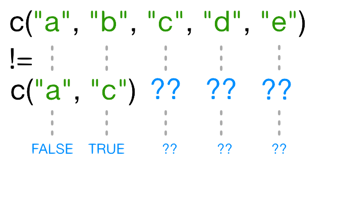
When one vector is shorter than the other, it gets recycled:
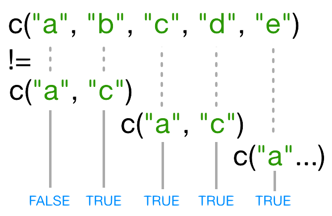
In this case R repeats c("a", "c") as many times as necessary to match names(x), i.e. we get c("a","c","a","c","a"). Since the recycled "a"
doesn’t match the third element of names(x), the value of != is TRUE.
Because in this case the longer vector length (5) isn’t a multiple of the shorter vector length (2), R printed a warning message. If we had been unlucky and names(x) had contained six elements, R would silently have done the wrong thing (i.e., not what we intended it to do). This recycling rule can can introduce hard-to-find and subtle bugs!
The way to get R to do what we really want (match each element of the left argument with all of the elements of the right argument) it to use the %in% operator. The %in% operator goes through each element of its left argument, in this case the names of x, and asks, “Does this element occur in the second argument?”. Here, since we want to exclude values, we also need a ! operator to change “in” to “not in”:
x[! names(x) %in% c("a","c") ]
  b   d   e
6.2 4.8 7.5
Challenge 3
Selecting elements of a vector that match any of a list of components is a very common data analysis task. For example, the gapminder data set contains
countryandcontinentvariables, but no information between these two scales. Suppose we want to pull out information from southeast Asia: how do we set up an operation to produce a logical vector that isTRUEfor all of the countries in southeast Asia andFALSEotherwise?Suppose you have these data:
seAsia <- c("Myanmar","Thailand","Cambodia","Vietnam","Laos")
## read in the gapminder data that we downloaded in episode 2
gapminder <- read.csv("data/gapminder_data.csv", header=TRUE)
## extract the `country` column from a data frame (we'll see this later);
## convert from a factor to a character;
## and get just the non-repeated elements
countries <- unique(as.character(gapminder$country))
There’s a wrong way (using only
==), which will give you a warning; a clunky way (using the logical operators==and|); and an elegant way (using%in%). See whether you can come up with all three and explain how they (don’t) work.Solution to challenge 3
- The wrong way to do this problem is
countries==seAsia. This gives a warning ("In countries == seAsia : longer object length is not a multiple of shorter object length") and the wrong answer (a vector of allFALSEvalues), because none of the recycled values ofseAsiahappen to line up correctly with matching values incountry.- The clunky (but technically correct) way to do this problem is
 (countries=="Myanmar" | countries=="Thailand" |
 countries=="Cambodia" | countries == "Vietnam" | countries=="Laos")
(or
countries==seAsia[1] | countries==seAsia[2] | ...). This gives the correct values, but hopefully you can see how awkward it is (what if we wanted to select countries from a much longer list?).
- The best way to do this problem is
countries %in% seAsia, which is both correct and easy to type (and read).
Handling special values
At some point you will encounter functions in R that cannot handle missing, infinite, or undefined data.
There are a number of special functions you can use to filter out this data:
is.nawill return all positions in a vector, matrix, or data.frame containingNA(orNaN)- likewise,
is.nan, andis.infinitewill do the same forNaNandInf. is.finitewill return all positions in a vector, matrix, or data.frame that do not containNA,NaNorInf.na.omitwill filter out all missing values from a vector
Factor subsetting
Now that we’ve explored the different ways to subset vectors, how do we subset the other data structures?
Factor subsetting works the same way as vector subsetting.
f <- factor(c("a", "a", "b", "c", "c", "d"))
f[f == "a"]
[1] a a
Levels: a b c d
f[f %in% c("b", "c")]
[1] b c c
Levels: a b c d
f[1:3]
[1] a a b
Levels: a b c d
Skipping elements will not remove the level even if no more of that category exists in the factor:
f[-3]
[1] a a c c d
Levels: a b c d
Tip: Higher dimensional arrays
when dealing with multi-dimensional arrays, each argument to
[corresponds to a dimension. For example, a 3D array, the first three arguments correspond to the rows, columns, and depth dimension.
List subsetting
Now we’ll introduce some new subsetting operators. There are three functions
used to subset lists. We’ve already seen these when learning about atomic vectors and matrices: [, [[, and $.
Using [ will always return a list. If you want to subset a list, but not
extract an element, then you will likely use [.
xlist <- list(a = "Software Carpentry", b = 1:10, data = head(mtcars))
xlist[1]
$a
[1] "Software Carpentry"
This returns a list with one element.
We can subset elements of a list exactly the same way as atomic
vectors using [. Comparison operations however won’t work as
they’re not recursive, they will try to condition on the data structures
in each element of the list, not the individual elements within those
data structures.
xlist[1:2]
$a
[1] "Software Carpentry"

$b
 [1]  1  2  3  4  5  6  7  8  9 10
To extract individual elements of a list, you need to use the double-square
bracket function: [[.
xlist[[1]]
[1] "Software Carpentry"
Notice that now the result is a vector, not a list.
You can’t extract more than one element at once:
xlist[[1:2]]
Error in xlist[[1:2]]: subscript out of bounds
Nor use it to skip elements:
xlist[[-1]]
Error in xlist[[-1]]: invalid negative subscript in get1index <real>
But you can use names to both subset and extract elements:
xlist[["a"]]
[1] "Software Carpentry"
The $ function is a shorthand way for extracting elements by name:
xlist$data
                   mpg cyl disp  hp drat    wt  qsec vs am gear carb
Mazda RX4         21.0   6  160 110 3.90 2.620 16.46  0  1    4    4
Mazda RX4 Wag     21.0   6  160 110 3.90 2.875 17.02  0  1    4    4
Datsun 710        22.8   4  108  93 3.85 2.320 18.61  1  1    4    1
Hornet 4 Drive    21.4   6  258 110 3.08 3.215 19.44  1  0    3    1
Hornet Sportabout 18.7   8  360 175 3.15 3.440 17.02  0  0    3    2
Valiant           18.1   6  225 105 2.76 3.460 20.22  1  0    3    1
Challenge 5
Given the following list:
xlist <- list(a = "Software Carpentry", b = 1:10, data = head(mtcars))Using your knowledge of both list and vector subsetting, extract the number 2 from xlist. Hint: the number 2 is contained within the “b” item in the list.
Solution to challenge 5
xlist$b[2][1] 2xlist[[2]][2][1] 2xlist[["b"]][2][1] 2
Challenge 6
Given a linear model:
mod <- aov(pop ~ lifeExp, data=gapminder)Extract the residual degrees of freedom (hint:
attributes()will help you)Solution to challenge 6
attributes(mod) ## `df.residual` is one of the names of `mod`mod$df.residual
Data frames
Remember the data frames are lists underneath the hood, so similar rules apply. However they are also two dimensional objects:
[ with one argument will act the same way as for lists, where each list
element corresponds to a column. The resulting object will be a data frame:
head(gapminder[3])
       pop
1  8425333
2  9240934
3 10267083
4 11537966
5 13079460
6 14880372
Similarly, [[ will act to extract a single column:
head(gapminder[["lifeExp"]])
[1] 28.801 30.332 31.997 34.020 36.088 38.438
And $ provides a convenient shorthand to extract columns by name:
head(gapminder$year)
[1] 1952 1957 1962 1967 1972 1977
With two arguments, [ behaves the same way as for matrices:
gapminder[1:3,]
      country year      pop continent lifeExp gdpPercap
1 Afghanistan 1952  8425333      Asia  28.801  779.4453
2 Afghanistan 1957  9240934      Asia  30.332  820.8530
3 Afghanistan 1962 10267083      Asia  31.997  853.1007
If we subset a single row, the result will be a data frame (because the elements are mixed types):
gapminder[3,]
      country year      pop continent lifeExp gdpPercap
3 Afghanistan 1962 10267083      Asia  31.997  853.1007
But for a single column the result will be a vector (this can
be changed with the third argument, drop = FALSE).
Challenge 7
Fix each of the following common data frame subsetting errors:
Extract observations collected for the year 1957
gapminder[gapminder$year = 1957,]Extract all columns except 1 through to 4
gapminder[,-1:4]Extract the rows where the life expectancy is longer the 80 years
gapminder[gapminder$lifeExp > 80]Extract the first row, and the fourth and fifth columns (
continentandlifeExp).gapminder[1, 4, 5]Advanced: extract rows that contain information for the years 2002 and 2007
gapminder[gapminder$year == 2002 | 2007,]Solution to challenge 7
Fix each of the following common data frame subsetting errors:
Extract observations collected for the year 1957
# gapminder[gapminder$year = 1957,]
gapminder[gapminder$year == 1957,]
Extract all columns except 1 through to 4
# gapminder[,-1:4]
gapminder[,-c(1:4)]
Extract the rows where the life expectancy is longer than 80 years
# gapminder[gapminder$lifeExp > 80]
gapminder[gapminder$lifeExp > 80,]
Extract the first row, and the fourth and fifth columns (
continentandlifeExp).# gapminder[1, 4, 5] gapminder[1, c(4, 5)]Advanced: extract rows that contain information for the years 2002 and 2007
 # gapminder[gapminder$year == 2002 | 2007,]
 gapminder[gapminder$year == 2002 | gapminder$year == 2007,]
 gapminder[gapminder$year %in% c(2002, 2007),]
Challenge 8
Why does
gapminder[1:20]return an error? How does it differ fromgapminder[1:20, ]?Create a new
data.framecalledgapminder_smallthat only contains rows 1 through 9 and 19 through 23. You can do this in one or two steps.Solution to challenge 8
gapminderis a data.frame so needs to be subsetted on two dimensions.gapminder[1:20, ]subsets the data to give the first 20 rows and all columns.2.
gapminder_small <- gapminder[c(1:9, 19:23),]
Key Points
Indexing in R starts at 1, not 0.
Access individual values by location using
[].Access slices of data using
[low:high].Access arbitrary sets of data using
[c(...)].Use logical operations and logical vectors to access subsets of data.
Data Frame Manipulation with dplyr
Overview
Teaching: 40 min
Exercises: 15 minQuestions
How can I manipulate data frames without repeating myself?
Objectives
To be able to use the six main data frame manipulation ‘verbs’ with pipes in
dplyr.To understand how
group_by()andsummarize()can be combined to summarize datasets.Be able to analyze a subset of data using logical filtering.
Manipulation of data frames means many things to many researchers, we often select certain observations (rows) or variables (columns), we often group the data by a certain variable(s), or we even calculate summary statistics. We can do these operations using the normal base R operations:
mean(gapminder[gapminder$continent == "Africa", "gdpPercap"])
[1] 2193.755
mean(gapminder[gapminder$continent == "Americas", "gdpPercap"])
[1] 7136.11
mean(gapminder[gapminder$continent == "Asia", "gdpPercap"])
[1] 7902.15
But this isn’t very nice because there is a fair bit of repetition. Repeating yourself will cost you time, both now and later, and potentially introduce some nasty bugs.
The dplyr package
Luckily, the dplyr
package provides a number of very useful functions for manipulating data frames
in a way that will reduce the above repetition, reduce the probability of making
errors, and probably even save you some typing. As an added bonus, you might
even find the dplyr grammar easier to read.
Tip: Tidyverse
dplyrpackage belongs to a broader family of opinionated R packages specifically designed for data science called “Tidyverse”. Some of these packages will be covered along this course, but you can find more complete information here: https://www.tidyverse.org/.
Here we’re going to cover 5 of the most commonly used functions as well as using
pipes (%>%) to combine them.
select()filter()group_by()summarize()mutate()
If you have have not installed this package earlier, please do so:
install.packages('dplyr')
Now let’s load the package:
library("dplyr")
Using select()
If, for example, we wanted to move forward with only a few of the variables in
our data frame we could use the select() function. This will keep only the
variables you select.
year_country_gdp <- select(gapminder, year, country, gdpPercap)
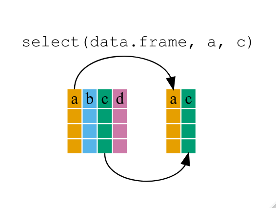 If we want to remove one column only from the
 gapminder data, for example,
removing the continent column.
smaller_gapminder_data <- select(gapminder, -continent)
If we open up year_country_gdp we’ll see that it only contains the year,
country and gdpPercap. Above we used ‘normal’ grammar, but the strengths of
dplyr lie in combining several functions using pipes. Since the pipes grammar
is unlike anything we’ve seen in R before, let’s repeat what we’ve done above
using pipes.
year_country_gdp <- gapminder %>% select(year, country, gdpPercap)
To help you understand why we wrote that in that way, let’s walk through it step
by step. First we summon the gapminder data frame and pass it on, using the pipe
symbol %>%, to the next step, which is the select() function. In this case
we don’t specify which data object we use in the select() function since in
gets that from the previous pipe. Fun Fact: There is a good chance you have
encountered pipes before in the shell. In R, a pipe symbol is %>% while in the
shell it is | but the concept is the same!
Tip: Renaming data frame columns in dplyr
In Chapter 4 we covered how you can rename columns with base R by assigning a value to the output of the
names()function. Just like select, this is a bit cumbersome, but thankfully dplyr has arename()function.Within a pipeline, the syntax is
rename(new_name = old_name). For example, we may want to rename the gdpPercap column name from ourselect()statement above.tidy_gdp <- year_country_gdp %>% rename(gdp_per_capita = gdpPercap) head(tidy_gdp)year country gdp_per_capita 1 1952 Afghanistan 779.4453 2 1957 Afghanistan 820.8530 3 1962 Afghanistan 853.1007 4 1967 Afghanistan 836.1971 5 1972 Afghanistan 739.9811 6 1977 Afghanistan 786.1134
Using filter()
If we now want to move forward with the above, but only with European
countries, we can combine select and filter
year_country_gdp_euro <- gapminder %>%
    filter(continent == "Europe") %>%
    select(year, country, gdpPercap)
If we now want to show life expectancy of European countries but only for a specific year (e.g., 2007), we can do as below.
europe_lifeExp_2007 <- gapminder %>%
  filter(continent == "Europe", year == 2007) %>%
  select(country, lifeExp)
Challenge 1
Write a single command (which can span multiple lines and includes pipes) that will produce a data frame that has the African values for
lifeExp,countryandyear, but not for other Continents. How many rows does your data frame have and why?Solution to Challenge 1
year_country_lifeExp_Africa <- gapminder %>%
                           filter(continent == "Africa") %>%
                           select(year, country, lifeExp)
As with last time, first we pass the gapminder data frame to the filter()
function, then we pass the filtered version of the gapminder data frame to the
select() function. Note: The order of operations is very important in this
case. If we used ‘select’ first, filter would not be able to find the variable
continent since we would have removed it in the previous step.
Using group_by()
Now, we were supposed to be reducing the error prone repetitiveness of what can
be done with base R, but up to now we haven’t done that since we would have to
repeat the above for each continent. Instead of filter(), which will only pass
observations that meet your criteria (in the above: continent=="Europe"), we
can use group_by(), which will essentially use every unique criteria that you
could have used in filter.
str(gapminder)
'data.frame':	1704 obs. of  6 variables:
 $ country  : chr  "Afghanistan" "Afghanistan" "Afghanistan" "Afghanistan" ...
 $ year     : int  1952 1957 1962 1967 1972 1977 1982 1987 1992 1997 ...
 $ pop      : num  8425333 9240934 10267083 11537966 13079460 ...
 $ continent: chr  "Asia" "Asia" "Asia" "Asia" ...
 $ lifeExp  : num  28.8 30.3 32 34 36.1 ...
 $ gdpPercap: num  779 821 853 836 740 ...
str(gapminder %>% group_by(continent))
gropd_df [1,704 × 6] (S3: grouped_df/tbl_df/tbl/data.frame)
 $ country  : chr [1:1704] "Afghanistan" "Afghanistan" "Afghanistan" "Afghanistan" ...
 $ year     : int [1:1704] 1952 1957 1962 1967 1972 1977 1982 1987 1992 1997 ...
 $ pop      : num [1:1704] 8425333 9240934 10267083 11537966 13079460 ...
 $ continent: chr [1:1704] "Asia" "Asia" "Asia" "Asia" ...
 $ lifeExp  : num [1:1704] 28.8 30.3 32 34 36.1 ...
 $ gdpPercap: num [1:1704] 779 821 853 836 740 ...
 - attr(*, "groups")= tibble [5 × 2] (S3: tbl_df/tbl/data.frame)
  ..$ continent: chr [1:5] "Africa" "Americas" "Asia" "Europe" ...
  ..$ .rows    : list<int> [1:5]
  .. ..$ : int [1:624] 25 26 27 28 29 30 31 32 33 34 ...
  .. ..$ : int [1:300] 49 50 51 52 53 54 55 56 57 58 ...
  .. ..$ : int [1:396] 1 2 3 4 5 6 7 8 9 10 ...
  .. ..$ : int [1:360] 13 14 15 16 17 18 19 20 21 22 ...
  .. ..$ : int [1:24] 61 62 63 64 65 66 67 68 69 70 ...
  .. ..@ ptype: int(0)
  ..- attr(*, ".drop")= logi TRUE
You will notice that the structure of the data frame where we used group_by()
(grouped_df) is not the same as the original gapminder (data.frame). A
grouped_df can be thought of as a list where each item in the listis a
data.frame which contains only the rows that correspond to the a particular
value continent (at least in the example above).
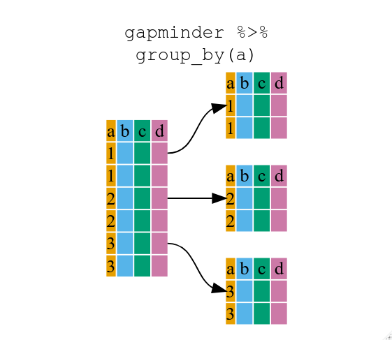
Using summarize()
The above was a bit on the uneventful side but group_by() is much more
exciting in conjunction with summarize(). This will allow us to create new
variable(s) by using functions that repeat for each of the continent-specific
data frames. That is to say, using the group_by() function, we split our
original data frame into multiple pieces, then we can run functions
(e.g. mean() or sd()) within summarize().
gdp_bycontinents <- gapminder %>%
    group_by(continent) %>%
    summarize(mean_gdpPercap = mean(gdpPercap))
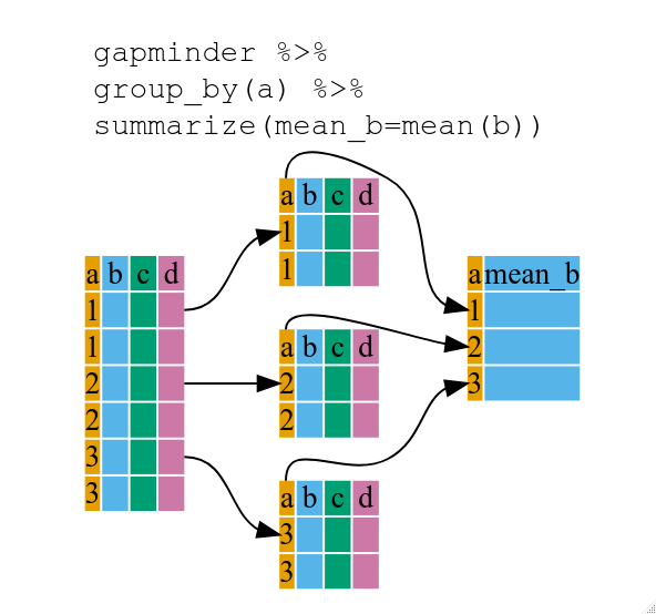
continent mean_gdpPercap
     <fctr>          <dbl>
1    Africa       2193.755
2  Americas       7136.110
3      Asia       7902.150
4    Europe      14469.476
5   Oceania      18621.609
That allowed us to calculate the mean gdpPercap for each continent, but it gets even better.
Challenge 2
Calculate the average life expectancy per country. Which has the longest average life expectancy and which has the shortest average life expectancy?
Solution to Challenge 2
lifeExp_bycountry <- gapminder %>%
   group_by(country) %>%
   summarize(mean_lifeExp = mean(lifeExp))
lifeExp_bycountry %>%
   filter(mean_lifeExp == min(mean_lifeExp) | mean_lifeExp == max(mean_lifeExp))
# A tibble: 2 × 2 country mean_lifeExp <chr> <dbl> 1 Iceland 76.5 2 Sierra Leone 36.8Another way to do this is to use the
dplyrfunctionarrange(), which arranges the rows in a data frame according to the order of one or more variables from the data frame. It has similar syntax to other functions from thedplyrpackage. You can usedesc()insidearrange()to sort in descending order.lifeExp_bycountry %>% arrange(mean_lifeExp) %>% head(1)# A tibble: 1 × 2 country mean_lifeExp <chr> <dbl> 1 Sierra Leone 36.8lifeExp_bycountry %>% arrange(desc(mean_lifeExp)) %>% head(1)# A tibble: 1 × 2 country mean_lifeExp <chr> <dbl> 1 Iceland 76.5Alphabetical order works too
lifeExp_bycountry %>%
   arrange(desc(country)) %>%
   head(1)
# A tibble: 1 × 2 country mean_lifeExp <chr> <dbl> 1 Zimbabwe 52.7
The function group_by() allows us to group by multiple variables. Let’s group by year and continent.
gdp_bycontinents_byyear <- gapminder %>%
    group_by(continent, year) %>%
    summarize(mean_gdpPercap = mean(gdpPercap))
`summarise()` has grouped output by 'continent'. You can override using the
`.groups` argument.
That is already quite powerful, but it gets even better! You’re not limited to defining 1 new variable in summarize().
gdp_pop_bycontinents_byyear <- gapminder %>%
    group_by(continent, year) %>%
    summarize(mean_gdpPercap = mean(gdpPercap),
              sd_gdpPercap = sd(gdpPercap),
              mean_pop = mean(pop),
              sd_pop = sd(pop))
`summarise()` has grouped output by 'continent'. You can override using the
`.groups` argument.
count() and n()
A very common operation is to count the number of observations for each
group. The dplyr package comes with two related functions that help with this.
For instance, if we wanted to check the number of countries included in the
dataset for the year 2002, we can use the count() function. It takes the name
of one or more columns that contain the groups we are interested in, and we can
optionally sort the results in descending order by adding sort=TRUE:
gapminder %>%
    filter(year == 2002) %>%
    count(continent, sort = TRUE)
  continent  n
1    Africa 52
2      Asia 33
3    Europe 30
4  Americas 25
5   Oceania  2
If we need to use the number of observations in calculations, the n() function
is useful. It will return the total number of observations in the current group rather than counting the number of observations in each group within a specific column. For instance, if we wanted to get the standard error of the life expectency per continent:
gapminder %>%
    group_by(continent) %>%
    summarize(se_le = sd(lifeExp)/sqrt(n()))
# A tibble: 5 × 2
  continent se_le
  <chr>     <dbl>
1 Africa    0.366
2 Americas  0.540
3 Asia      0.596
4 Europe    0.286
5 Oceania   0.775
You can also chain together several summary operations; in this case calculating the minimum, maximum, mean and se of each continent’s per-country life-expectancy:
gapminder %>%
    group_by(continent) %>%
    summarize(
      mean_le = mean(lifeExp),
      min_le = min(lifeExp),
      max_le = max(lifeExp),
      se_le = sd(lifeExp)/sqrt(n()))
# A tibble: 5 × 5
  continent mean_le min_le max_le se_le
  <chr>       <dbl>  <dbl>  <dbl> <dbl>
1 Africa       48.9   23.6   76.4 0.366
2 Americas     64.7   37.6   80.7 0.540
3 Asia         60.1   28.8   82.6 0.596
4 Europe       71.9   43.6   81.8 0.286
5 Oceania      74.3   69.1   81.2 0.775
Using mutate()
We can also create new variables prior to (or even after) summarizing information using mutate().
gdp_pop_bycontinents_byyear <- gapminder %>%
    mutate(gdp_billion = gdpPercap*pop/10^9) %>%
    group_by(continent,year) %>%
    summarize(mean_gdpPercap = mean(gdpPercap),
              sd_gdpPercap = sd(gdpPercap),
              mean_pop = mean(pop),
              sd_pop = sd(pop),
              mean_gdp_billion = mean(gdp_billion),
              sd_gdp_billion = sd(gdp_billion))
`summarise()` has grouped output by 'continent'. You can override using the
`.groups` argument.
Connect mutate with logical filtering: ifelse
When creating new variables, we can hook this with a logical condition. A simple combination of
mutate() and ifelse() facilitates filtering right where it is needed: in the moment of creating something new.
This easy-to-read statement is a fast and powerful way of discarding certain data (even though the overall dimension
of the data frame will not change) or for updating values depending on this given condition.
## keeping all data but "filtering" after a certain condition
# calculate GDP only for people with a life expectation above 25
gdp_pop_bycontinents_byyear_above25 <- gapminder %>%
    mutate(gdp_billion = ifelse(lifeExp > 25, gdpPercap * pop / 10^9, NA)) %>%
    group_by(continent, year) %>%
    summarize(mean_gdpPercap = mean(gdpPercap),
              sd_gdpPercap = sd(gdpPercap),
              mean_pop = mean(pop),
              sd_pop = sd(pop),
              mean_gdp_billion = mean(gdp_billion),
              sd_gdp_billion = sd(gdp_billion))
`summarise()` has grouped output by 'continent'. You can override using the
`.groups` argument.
## updating only if certain condition is fullfilled
# for life expectations above 40 years, the gpd to be expected in the future is scaled
gdp_future_bycontinents_byyear_high_lifeExp <- gapminder %>%
    mutate(gdp_futureExpectation = ifelse(lifeExp > 40, gdpPercap * 1.5, gdpPercap)) %>%
    group_by(continent, year) %>%
    summarize(mean_gdpPercap = mean(gdpPercap),
              mean_gdpPercap_expected = mean(gdp_futureExpectation))
`summarise()` has grouped output by 'continent'. You can override using the
`.groups` argument.
Key Points
Use the
dplyrpackage to manipulate data frames.Use
select()to choose variables from a data frame.Use
filter()to choose data based on values.Use
group_by()andsummarize()to work with subsets of data.Use
mutate()to create new variables.
Creating Publication-Quality Graphics with ggplot2
Overview
Teaching: 60 min
Exercises: 20 minQuestions
How can I create publication-quality graphics in R?
Objectives
To be able to use ggplot2 to generate publication-quality graphics.
To apply geometry, aesthetic, and statistics layers to a ggplot plot.
To manipulate the aesthetics of a plot using different colors, shapes, and lines.
To improve data visualization through transforming scales and paneling by group.
To save a plot created with ggplot to disk.
Plotting our data is one of the best ways to quickly explore it and the various relationships between variables.
There are three main plotting systems in R, the base plotting system, the lattice package, and the ggplot2 package.
Today we’ll be learning about the ggplot2 package, because it is the most effective for creating publication-quality graphics.
ggplot2 is built on the grammar of graphics, the idea that any plot can be expressed from the same set of components: a data set, a coordinate system, and a set of geoms – the visual representation of data points.
The key to understanding ggplot2 is thinking about a figure in layers. This idea may be familiar to you if you have used image editing programs like Photoshop, Illustrator, or Inkscape.
Let’s start off with an example:
library("ggplot2")
ggplot(data = gapminder, mapping = aes(x = gdpPercap, y = lifeExp)) +
  geom_point()
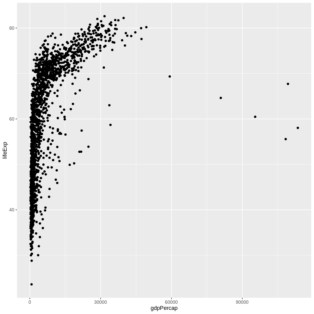
So the first thing we do is call the ggplot function. This function lets R
know that we’re creating a new plot, and any of the arguments we give the
ggplot function are the global options for the plot: they apply to all
layers on the plot.
We’ve passed in two arguments to ggplot. First, we tell ggplot what data we
want to show on our figure, in this example the gapminder data we read in
earlier. For the second argument, we passed in the aes function, which
tells ggplot how variables in the data map to aesthetic properties of
the figure, in this case the x and y locations. Here we told ggplot we
want to plot the “gdpPercap” column of the gapminder data frame on the x-axis, and
the “lifeExp” column on the y-axis. Notice that we didn’t need to explicitly
pass aes these columns (e.g. x = gapminder[, "gdpPercap"]), this is because
ggplot is smart enough to know to look in the data for that column!
By itself, the call to ggplot isn’t enough to draw a figure:
ggplot(data = gapminder, mapping = aes(x = gdpPercap, y = lifeExp))
We need to tell ggplot how we want to visually represent the data, which we
do by adding a new geom layer. In our example, we used geom_point, which
tells ggplot we want to visually represent the relationship between x and
y as a scatterplot of points:
ggplot(data = gapminder, mapping = aes(x = gdpPercap, y = lifeExp)) +
  geom_point()

Challenge 1
Modify the example so that the figure shows how life expectancy has changed over time:
ggplot(data = gapminder, mapping = aes(x = gdpPercap, y = lifeExp)) + geom_point()Hint: the gapminder dataset has a column called “year”, which should appear on the x-axis.
Solution to challenge 1
Here is one possible solution:
ggplot(data = gapminder, mapping = aes(x = year, y = lifeExp)) + geom_point()
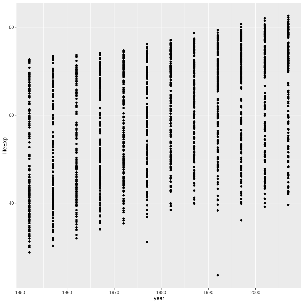
Challenge 2
In the previous examples and challenge we’ve used the
aesfunction to tell the scatterplot geom about the x and y locations of each point. Another aesthetic property we can modify is the point color. Modify the code from the previous challenge to color the points by the “continent” column. What trends do you see in the data? Are they what you expected?Solution to challenge 2
The solution presented below adds
color=continentto the call of theaesfunction. The general trend seems to indicate an increased life expectancy over the years. On continents with stronger economies we find a longer life expectancy.ggplot(data = gapminder, mapping = aes(x = year, y = lifeExp, color=continent)) + geom_point()
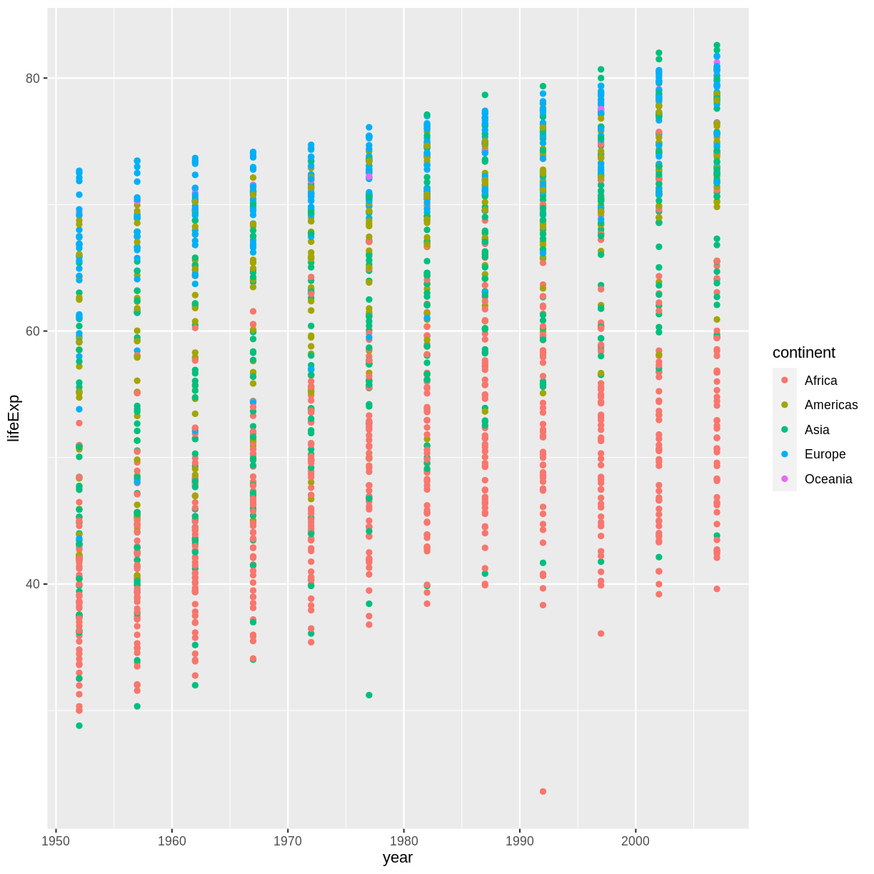
Layers
Using a scatterplot probably isn’t the best for visualizing change over time.
Instead, let’s tell ggplot to visualize the data as a line plot:
ggplot(data = gapminder, mapping = aes(x=year, y=lifeExp, color=continent)) +
  geom_line()
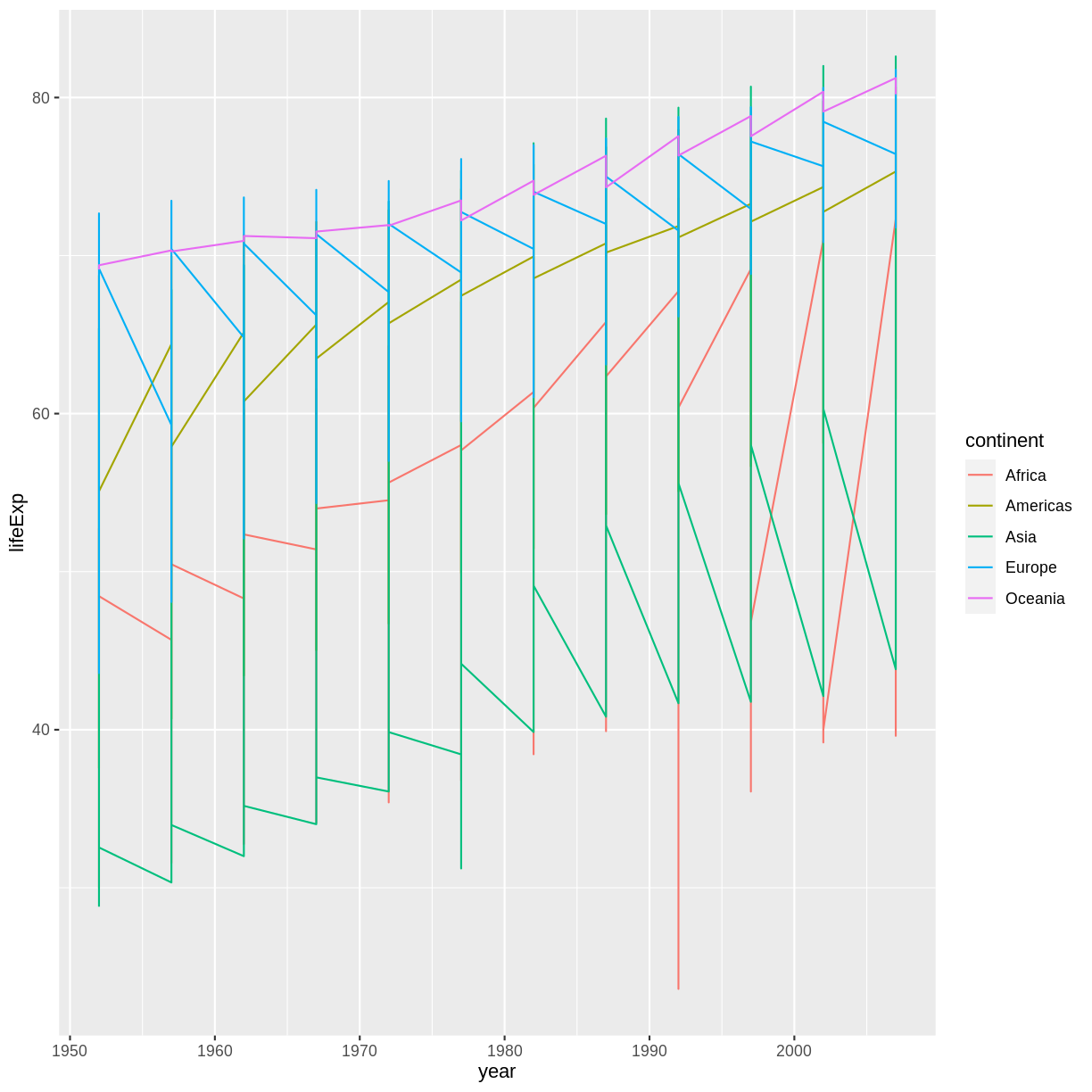
Instead of adding a geom_point layer, we’ve added a geom_line layer.
However, the result doesn’t look quite as we might have expected: it seems to be jumping around a lot in each continent. Let’s try to separate the data by country, plotting one line for each country:
ggplot(data = gapminder, mapping = aes(x=year, y=lifeExp, by=country, color=continent)) +
  geom_line()
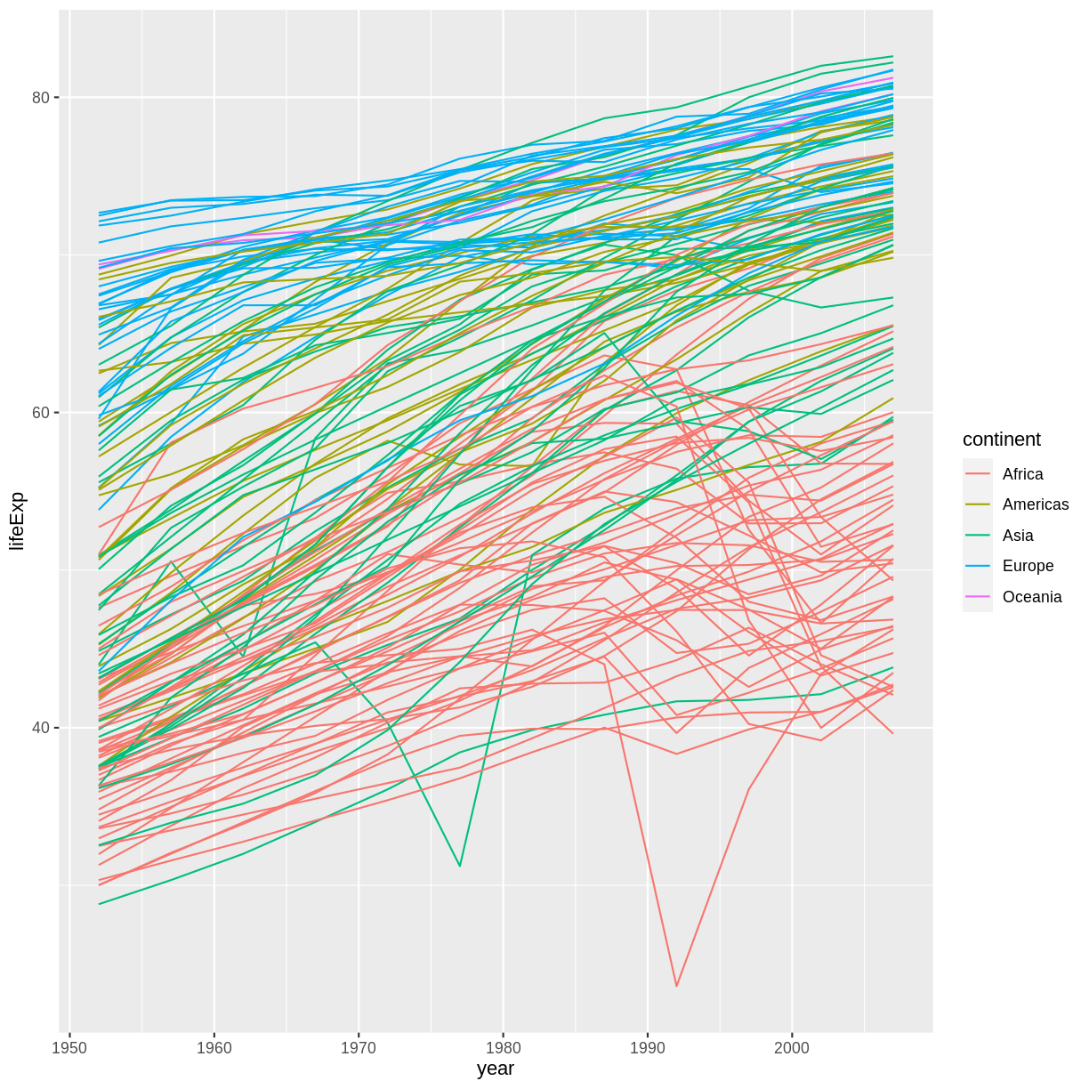
We’ve added the by aesthetic, which tells ggplot to draw a line for each
country.
But what if we want to visualize both lines and points on the plot? We can add another layer to the plot:
ggplot(data = gapminder, mapping = aes(x=year, y=lifeExp, by=country, color=continent)) +
  geom_line() + geom_point()

It’s important to note that each layer is drawn on top of the previous layer. In this example, the points have been drawn on top of the lines. Here’s a demonstration:
ggplot(data = gapminder, mapping = aes(x=year, y=lifeExp, by=country)) +
  geom_line(mapping = aes(color=continent)) + geom_point()
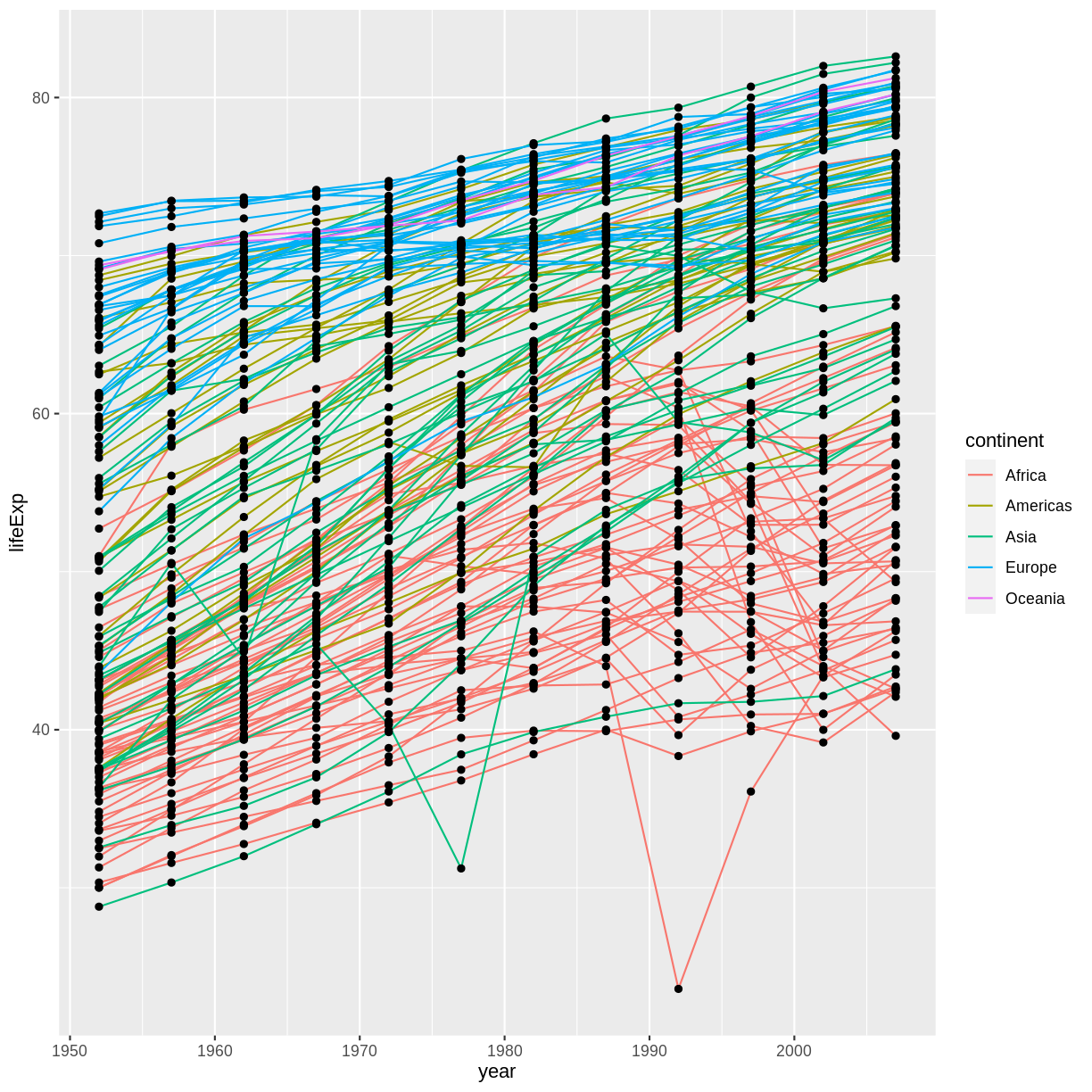
In this example, the aesthetic mapping of color has been moved from the
global plot options in ggplot to the geom_line layer so it no longer applies
to the points. Now we can clearly see that the points are drawn on top of the
lines.
Tip: Setting an aesthetic to a value instead of a mapping
So far, we’ve seen how to use an aesthetic (such as color) as a mapping to a variable in the data. For example, when we use
geom_line(mapping = aes(color=continent)), ggplot will give a different color to each continent. But what if we want to change the color of all lines to blue? You may think thatgeom_line(mapping = aes(color="blue"))should work, but it doesn’t. Since we don’t want to create a mapping to a specific variable, we can move the color specification outside of theaes()function, like this:geom_line(color="blue").
Challenge 3
Switch the order of the point and line layers from the previous example. What happened?
Solution to challenge 3
The lines now get drawn over the points!
ggplot(data = gapminder, mapping = aes(x=year, y=lifeExp, by=country)) +
 geom_point() + geom_line(mapping = aes(color=continent))
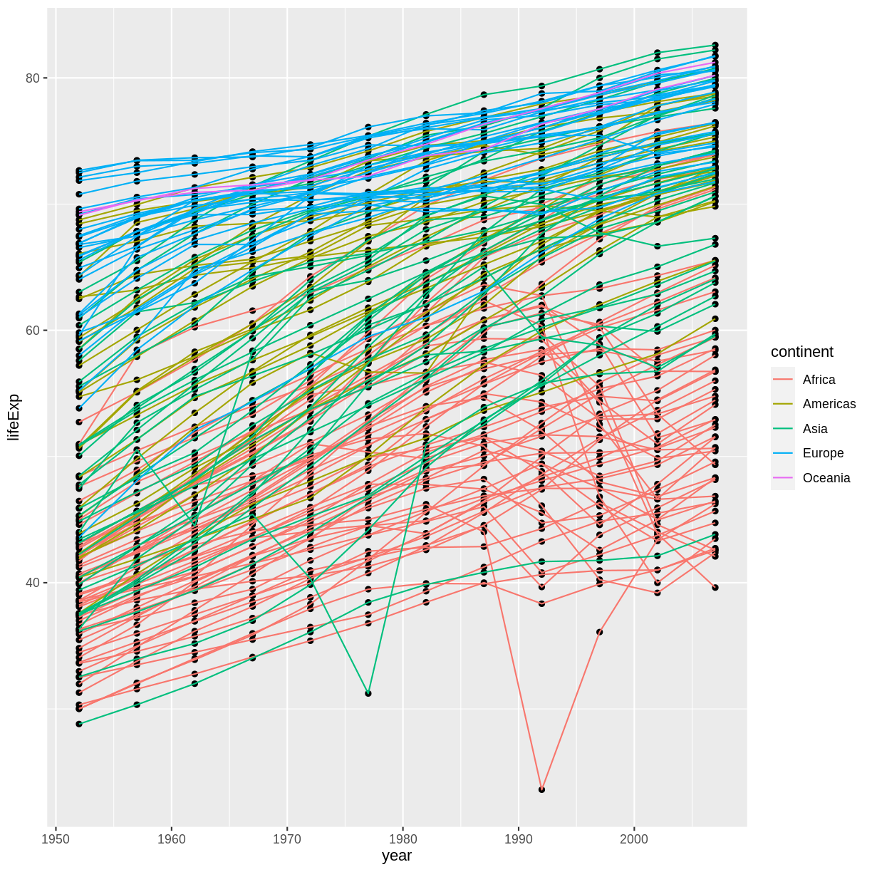
Transformations and statistics
ggplot2 also makes it easy to overlay statistical models over the data. To demonstrate we’ll go back to our first example:
ggplot(data = gapminder, mapping = aes(x = gdpPercap, y = lifeExp)) +
geom_point()

Currently it’s hard to see the relationship between the points due to some strong outliers in GDP per capita. We can change the scale of units on the x axis using the scale functions. These control the mapping between the data values and visual values of an aesthetic. We can also modify the transparency of the points, using the alpha function, which is especially helpful when you have a large amount of data which is very clustered.
ggplot(data = gapminder, mapping = aes(x = gdpPercap, y = lifeExp)) +
geom_point(alpha = 0.5) + scale_x_log10()
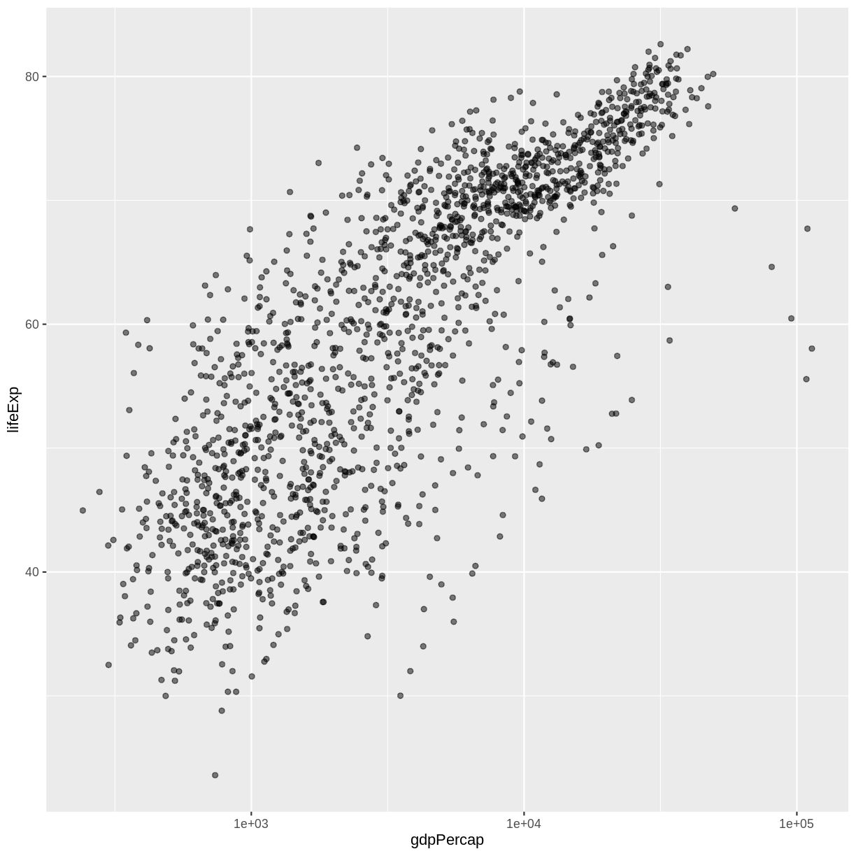
The scale_x_log10 function applied a transformation to the coordinate system of the plot, so that each multiple of 10 is evenly spaced from left to right. For example, a GDP per capita of 1,000 is the same horizontal distance away from a value of 10,000 as the 10,000 value is from 100,000. This helps to visualize the spread of the data along the x-axis.
Tip Reminder: Setting an aesthetic to a value instead of a mapping
Notice that we used
geom_point(alpha = 0.5). As the previous tip mentioned, using a setting outside of theaes()function will cause this value to be used for all points, which is what we want in this case. But just like any other aesthetic setting, alpha can also be mapped to a variable in the data. For example, we can give a different transparency to each continent withgeom_point(mapping = aes(alpha = continent)).
We can fit a simple relationship to the data by adding another layer,
geom_smooth:
ggplot(data = gapminder, mapping = aes(x = gdpPercap, y = lifeExp)) +
geom_point(alpha = 0.5) + scale_x_log10() + geom_smooth(method="lm")
`geom_smooth()` using formula = 'y ~ x'
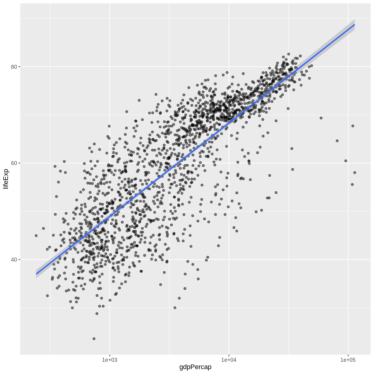
We can make the line thicker by setting the size aesthetic in the
geom_smooth layer:
ggplot(data = gapminder, mapping = aes(x = gdpPercap, y = lifeExp)) +
geom_point(alpha = 0.5) + scale_x_log10() + geom_smooth(method="lm", size=1.5)
Warning: Using `size` aesthetic for lines was deprecated in ggplot2 3.4.0.
ℹ Please use `linewidth` instead.
`geom_smooth()` using formula = 'y ~ x'
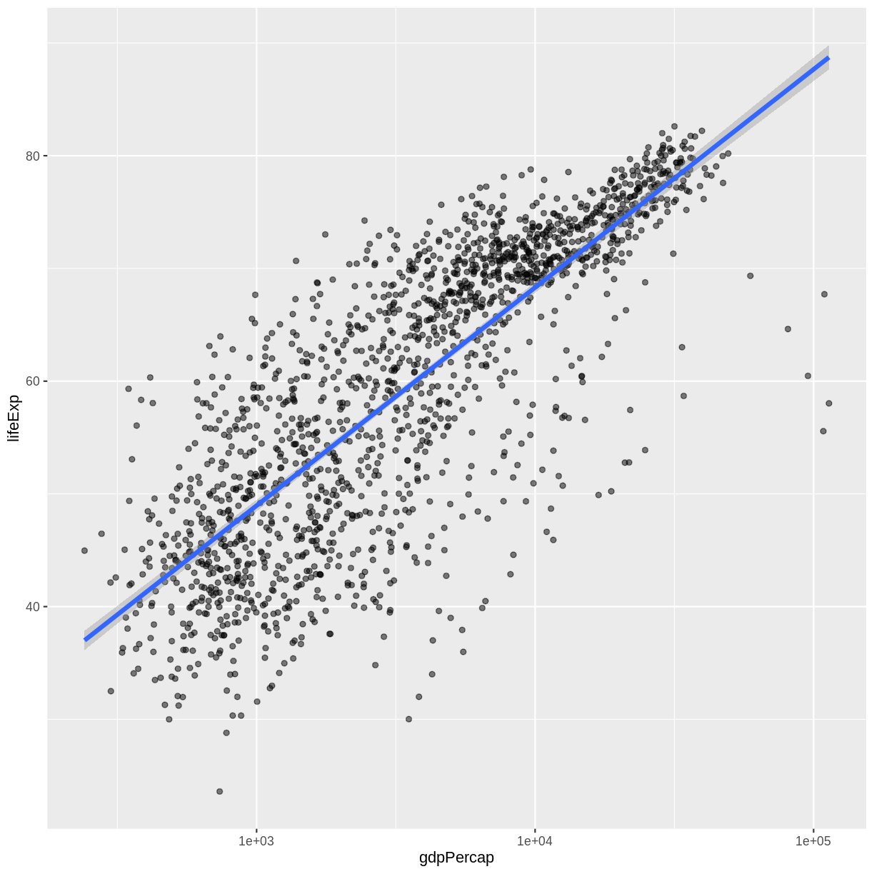
There are two ways an aesthetic can be specified. Here we set the size
aesthetic by passing it as an argument to geom_smooth. Previously in the
lesson we’ve used the aes function to define a mapping between data
variables and their visual representation.
Challenge 4a
Modify the color and size of the points on the point layer in the previous example.
Hint: do not use the
aesfunction.Solution to challenge 4a
Here a possible solution: Notice that the
colorargument is supplied outside of theaes()function. This means that it applies to all data points on the graph and is not related to a specific variable.ggplot(data = gapminder, mapping = aes(x = gdpPercap, y = lifeExp)) + geom_point(size=3, color="orange") + scale_x_log10() + geom_smooth(method="lm", size=1.5)`geom_smooth()` using formula = 'y ~ x'
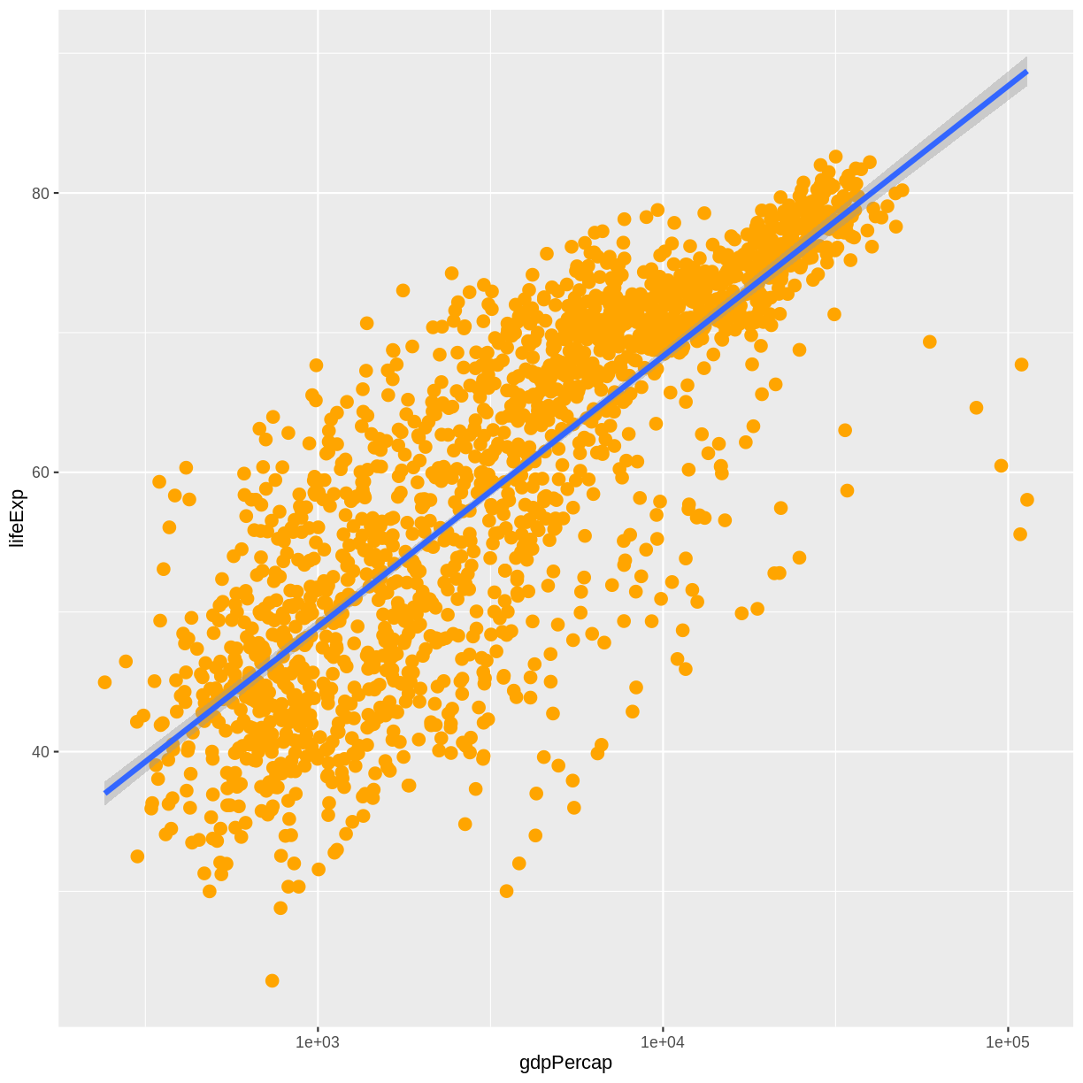
Challenge 4b
Modify your solution to Challenge 4a so that the points are now a different shape and are colored by continent with new trendlines. Hint: The color argument can be used inside the aesthetic.
Solution to challenge 4b
Here is a possible solution: Notice that supplying the
colorargument inside theaes()functions enables you to connect it to a certain variable. Theshapeargument, as you can see, modifies all data points the same way (it is outside theaes()call) while thecolorargument which is placed inside theaes()call modifies a point’s color based on its continent value.ggplot(data = gapminder, mapping = aes(x = gdpPercap, y = lifeExp, color = continent)) + geom_point(size=3, shape=17) + scale_x_log10() + geom_smooth(method="lm", size=1.5)`geom_smooth()` using formula = 'y ~ x'
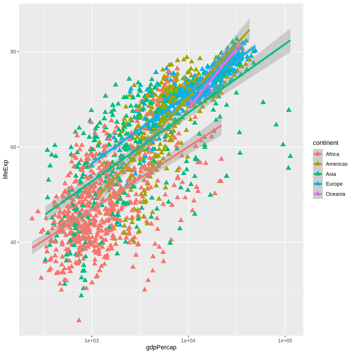
Multi-panel figures
Earlier we visualized the change in life expectancy over time across all countries in one plot. Alternatively, we can split this out over multiple panels by adding a layer of facet panels.
Tip
We start by making a subset of data including only countries located in the Americas. This includes 25 countries, which will begin to clutter the figure. Note that we apply a “theme” definition to rotate the x-axis labels to maintain readability. Nearly everything in ggplot2 is customizable.
americas <- gapminder[gapminder$continent == "Americas",]
ggplot(data = americas, mapping = aes(x = year, y = lifeExp)) +
geom_line() +
facet_wrap( ~ country) +
theme(axis.text.x = element_text(angle = 45))

The facet_wrap layer took a “formula” as its argument, denoted by the tilde
(~). This tells R to draw a panel for each unique value in the country column
of the gapminder dataset.
Modifying text
To clean this figure up for a publication we need to change some of the text elements. The x-axis is too cluttered, and the y axis should read “Life expectancy”, rather than the column name in the data frame.
We can do this by adding a couple of different layers. The theme layer
controls the axis text, and overall text size. Labels for the axes, plot
title and any legend can be set using the labs function. Legend titles
are set using the same names we used in the aes specification. Thus below
the color legend title is set using color = "Continent", while the title
of a fill legend would be set using fill = "MyTitle".
ggplot(data = americas, mapping = aes(x = year, y = lifeExp, color=continent)) +
geom_line() + facet_wrap( ~ country) +
labs(
x = "Year", # x axis title
y = "Life expectancy", # y axis title
title = "Figure 1", # main title of figure
color = "Continent" # title of legend
) +
theme(axis.text.x = element_text(angle = 90, hjust = 1))
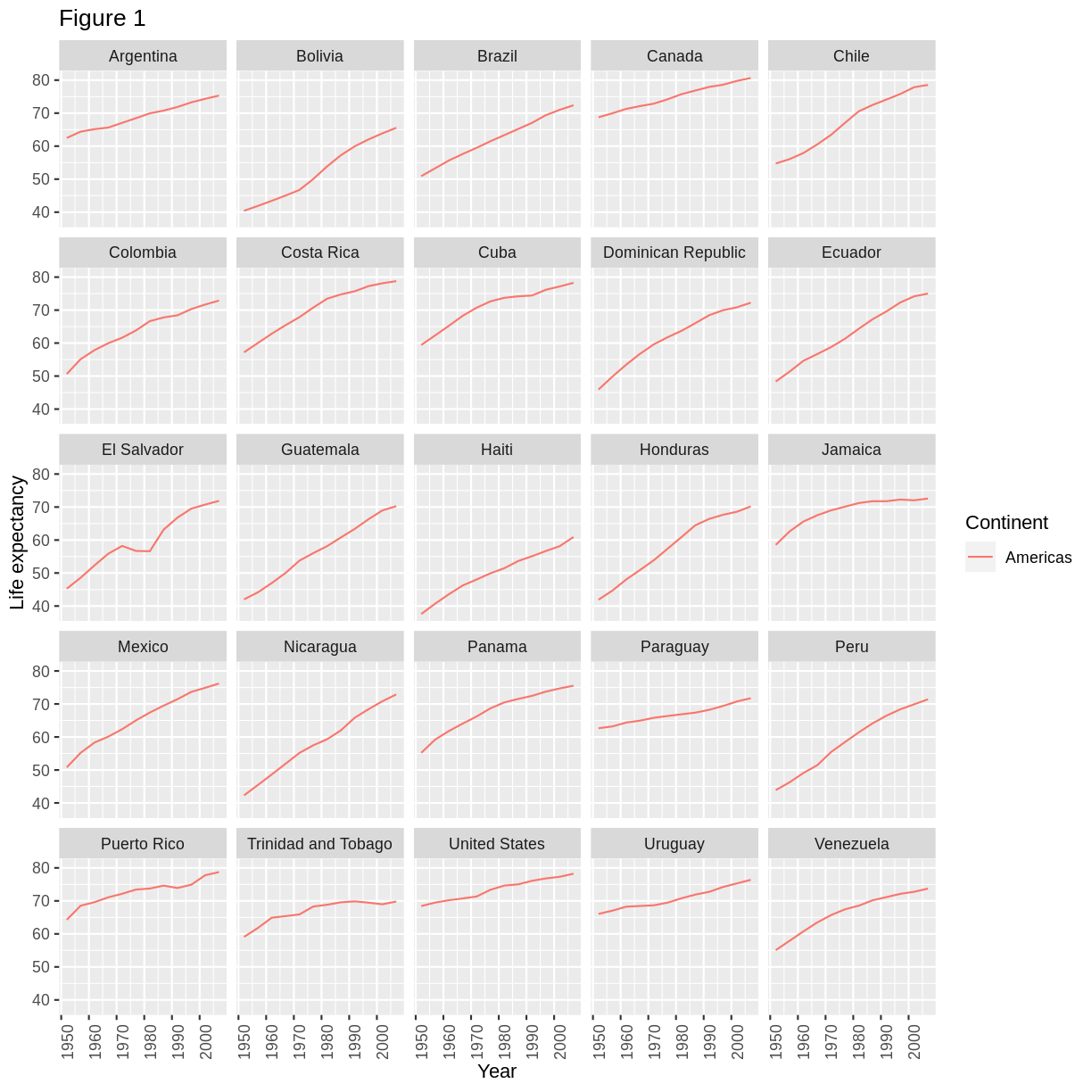
Exporting the plot
The ggsave() function allows you to export a plot created with ggplot. You can specify the dimension and resolution of your plot by adjusting the appropriate arguments (width, height and dpi) to create high quality graphics for publication. In order to save the plot from above, we first assign it to a variable lifeExp_plot, then tell ggsave to save that plot in png format to a directory called results. (Make sure you have a results/ folder in your working directory.)
lifeExp_plot <- ggplot(data = americas, mapping = aes(x = year, y = lifeExp, color=continent)) +
geom_line() + facet_wrap( ~ country) +
labs(
x = "Year", # x axis title
y = "Life expectancy", # y axis title
title = "Figure 1", # main title of figure
color = "Continent" # title of legend
) +
theme(axis.text.x = element_text(angle = 90, hjust = 1))
ggsave(filename = "results/lifeExp.png", plot = lifeExp_plot, width = 12, height = 10, dpi = 300, units = "cm")
There are two nice things about ggsave. First, it defaults to the last plot, so if you omit the plot argument it will automatically save the last plot you created with ggplot. Secondly, it tries to determine the format you want to save your plot in from the file extension you provide for the filename (for example .png or .pdf). If you need to, you can specify the format explicitly in the device argument.
This is a taste of what you can do with ggplot2. RStudio provides a really useful cheat sheet of the different layers available, and more extensive documentation is available on the ggplot2 website. Finally, if you have no idea how to change something, a quick Google search will usually send you to a relevant question and answer on Stack Overflow with reusable code to modify!
Challenge 5
Generate boxplots to compare life expectancy between the different continents during the available years.
Advanced:
- Rename y axis as Life Expectancy.
- Remove x axis labels.
Solution to Challenge 5
Here a possible solution:
xlab()andylab()set labels for the x and y axes, respectively The axis title, text and ticks are attributes of the theme and must be modified within atheme()call.ggplot(data = gapminder, mapping = aes(x = continent, y = lifeExp, fill = continent)) + geom_boxplot() + facet_wrap(~year) + ylab("Life Expectancy") + theme(axis.title.x=element_blank(), axis.text.x = element_blank(), axis.ticks.x = element_blank())
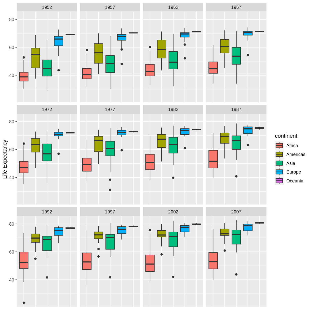
Key Points
Use
ggplot2to create plots.Think about graphics in layers: aesthetics, geometry, statistics, scale transformation, and grouping.
Combining ggplo2 and dplyr
Overview
Teaching: 15 min
Exercises: 15 minQuestions
How can I use ggplot2 and dplyr together?
Objectives
Use pipes (
%>%) to pass data toggplot()
Combining dplyr and ggplot2
First install and load ggplot2:
install.packages('ggplot2')
library("ggplot2")
In the plotting lesson we looked at how to make a multi-panel figure by adding
a layer of facet panels using ggplot2. Here is the code we used (with some
extra comments):
# Filter countries located in the Americas
americas <- gapminder[gapminder$continent == "Americas", ]
# Make the plot
ggplot(data = americas, mapping = aes(x = year, y = lifeExp)) +
geom_line() +
facet_wrap( ~ country) +
theme(axis.text.x = element_text(angle = 45))

This code makes the right plot but it also creates an intermediate variable
(americas) that we might not have any other uses for. Just as we used
%>% to pipe data along a chain of dplyr functions we can use it to pass data
to ggplot(). Because %>% replaces the first argument in a function we don’t
need to specify the data = argument in the ggplot() function. By combining
dplyr and ggplot2 functions we can make the same figure without creating any
new variables or modifying the data.
gapminder %>%
# Filter countries located in the Americas
filter(continent == "Americas") %>%
# Make the plot
ggplot(mapping = aes(x = year, y = lifeExp)) +
geom_line() +
facet_wrap( ~ country) +
theme(axis.text.x = element_text(angle = 45))

More examples of using the function mutate() and the ggplot2 package.
gapminder %>%
# extract first letter of country name into new column
mutate(startsWith = substr(country, 1, 1)) %>%
# only keep countries starting with A or Z
filter(startsWith %in% c("A", "Z")) %>%
# plot lifeExp into facets
ggplot(aes(x = year, y = lifeExp, colour = continent)) +
geom_line() +
facet_wrap(vars(country)) +
theme_minimal()
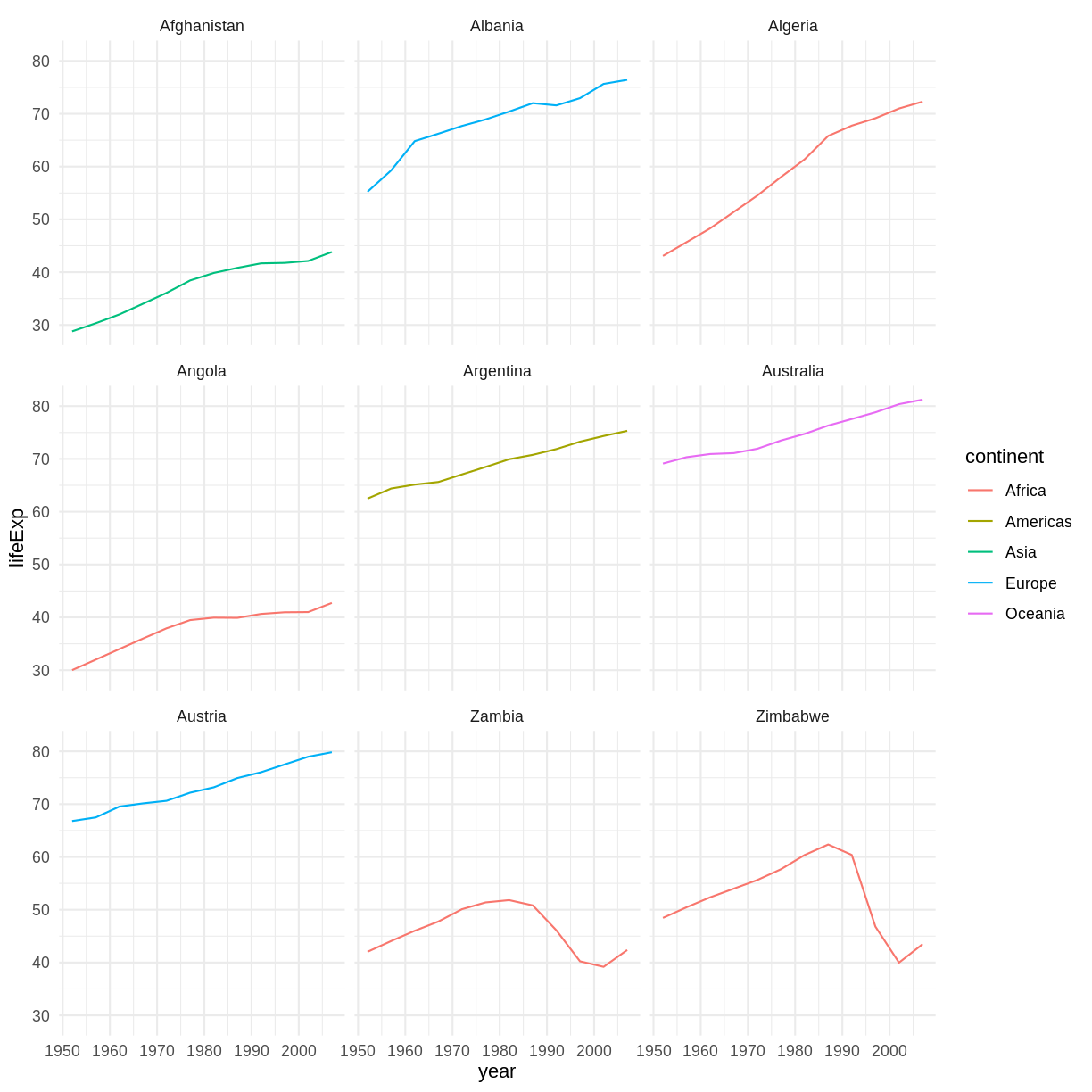
Advanced Challenge
Calculate the average life expectancy in 2002 of 2 randomly selected countries for each continent. Then arrange the continent names in reverse order. Hint: Use the
dplyrfunctionsarrange()andsample_n(), they have similar syntax to other dplyr functions.Solution to Advanced Challenge
lifeExp_2countries_bycontinents <- gapminder %>% filter(year==2002) %>% group_by(continent) %>% sample_n(2) %>% summarize(mean_lifeExp=mean(lifeExp)) %>% arrange(desc(mean_lifeExp))
Other great resources
- R for Data Science
- Data Wrangling Cheat sheet
- Introduction to dplyr
- Data wrangling with R and RStudio
Key Points
Use
ggplot2to create plots.Think about graphics in layers: aesthetics, geometry, statistics, scale transformation, and grouping.
Control Flow (extra)
Overview
Teaching: 0 min
Exercises: 0 minQuestions
How can I make data-dependent choices in R?
How can I repeat operations in R?
Objectives
Write conditional statements with
if...elsestatements andifelse().Write and understand
for()loops.
Often when we’re coding we want to control the flow of our actions. This can be done by setting actions to occur only if a condition or a set of conditions are met. Alternatively, we can also set an action to occur a particular number of times.
There are several ways you can control flow in R. For conditional statements, the most commonly used approaches are the constructs:
# if
if (condition is true) {
perform action
}
# if ... else
if (condition is true) {
perform action
} else { # that is, if the condition is false,
perform alternative action
}
Say, for example, that we want R to print a message if a variable x has a particular value:
x <- 8
if (x >= 10) {
print("x is greater than or equal to 10")
}
x
[1] 8
The print statement does not appear in the console because x is not greater than 10. To print a different message for numbers less than 10, we can add an else statement.
x <- 8
if (x >= 10) {
print("x is greater than or equal to 10")
} else {
print("x is less than 10")
}
[1] "x is less than 10"
You can also test multiple conditions by using else if.
x <- 8
if (x >= 10) {
print("x is greater than or equal to 10")
} else if (x > 5) {
print("x is greater than 5, but less than 10")
} else {
print("x is less than 5")
}
[1] "x is greater than 5, but less than 10"
Important: when R evaluates the condition inside if() statements, it is
looking for a logical element, i.e., TRUE or FALSE. This can cause some
headaches for beginners. For example:
x <- 4 == 3
if (x) {
"4 equals 3"
} else {
"4 does not equal 3"
}
[1] "4 does not equal 3"
As we can see, the not equal message was printed because the vector x is FALSE
x <- 4 == 3
x
[1] FALSE
Challenge 1
Use an
if()statement to print a suitable message reporting whether there are any records from 2002 in thegapminderdataset. Now do the same for 2012.Solution to Challenge 1
We will first see a solution to Challenge 1 which does not use the
any()function. We first obtain a logical vector describing which element ofgapminder$yearis equal to2002:gapminder[(gapminder$year == 2002),]Then, we count the number of rows of the data.frame
gapminderthat correspond to the 2002:rows2002_number <- nrow(gapminder[(gapminder$year == 2002),])The presence of any record for the year 2002 is equivalent to the request that
rows2002_numberis one or more:rows2002_number >= 1Putting all together, we obtain:
if(nrow(gapminder[(gapminder$year == 2002),]) >= 1){ print("Record(s) for the year 2002 found.") }All this can be done more quickly with
any(). The logical condition can be expressed as:if(any(gapminder$year == 2002)){ print("Record(s) for the year 2002 found.") }
Did anyone get a warning message like this?
Error in if (gapminder$year == 2012) {: the condition has length > 1
The if() function only accepts singular (of length 1) inputs, and therefore
returns an error when you use it with a vector. The if() function will still
run, but will only evaluate the condition in the first element of the vector.
Therefore, to use the if() function, you need to make sure your input is
singular (of length 1).
Tip: Built in
ifelse()function
Raccepts bothif()andelse if()statements structured as outlined above, but also statements usingR’s built-inifelse()function. This function accepts both singular and vector inputs and is structured as follows:# ifelse function ifelse(condition is true, perform action, perform alternative action)where the first argument is the condition or a set of conditions to be met, the second argument is the statement that is evaluated when the condition is
TRUE, and the third statement is the statement that is evaluated when the condition isFALSE.y <- -3 ifelse(y < 0, "y is a negative number", "y is either positive or zero")[1] "y is a negative number"
Tip:
any()andall()The
any()function will returnTRUEif at least oneTRUEvalue is found within a vector, otherwise it will returnFALSE. This can be used in a similar way to the%in%operator. The functionall(), as the name suggests, will only returnTRUEif all values in the vector areTRUE.
Repeating operations
If you want to iterate over
a set of values, when the order of iteration is important, and perform the
same operation on each, a for() loop will do the job.
We saw for() loops in the shell lessons earlier. This is the most
flexible of looping operations, but therefore also the hardest to use
correctly. In general, the advice of many R users would be to learn about
for() loops, but to avoid using for() loops unless the order of iteration is
important: i.e. the calculation at each iteration depends on the results of
previous iterations. If the order of iteration is not important, then you
should learn about vectorized alternatives, such as the purrr package, as they
pay off in computational efficiency.
The basic structure of a for() loop is:
for (iterator in set of values) {
do a thing
}
For example:
for (i in 1:10) {
print(i)
}
[1] 1
[1] 2
[1] 3
[1] 4
[1] 5
[1] 6
[1] 7
[1] 8
[1] 9
[1] 10
The 1:10 bit creates a vector on the fly; you can iterate
over any other vector as well.
We can use a for() loop nested within another for() loop to iterate over two things at
once.
for (i in 1:5) {
for (j in c('a', 'b', 'c', 'd', 'e')) {
print(paste(i,j))
}
}
[1] "1 a"
[1] "1 b"
[1] "1 c"
[1] "1 d"
[1] "1 e"
[1] "2 a"
[1] "2 b"
[1] "2 c"
[1] "2 d"
[1] "2 e"
[1] "3 a"
[1] "3 b"
[1] "3 c"
[1] "3 d"
[1] "3 e"
[1] "4 a"
[1] "4 b"
[1] "4 c"
[1] "4 d"
[1] "4 e"
[1] "5 a"
[1] "5 b"
[1] "5 c"
[1] "5 d"
[1] "5 e"
We notice in the output that when the first index (i) is set to 1, the second
index (j) iterates through its full set of indices. Once the indices of j
have been iterated through, then i is incremented. This process continues
until the last index has been used for each for() loop.
Rather than printing the results, we could write the loop output to a new object.
output_vector <- c()
for (i in 1:5) {
for (j in c('a', 'b', 'c', 'd', 'e')) {
temp_output <- paste(i, j)
output_vector <- c(output_vector, temp_output)
}
}
output_vector
[1] "1 a" "1 b" "1 c" "1 d" "1 e" "2 a" "2 b" "2 c" "2 d" "2 e" "3 a" "3 b"
[13] "3 c" "3 d" "3 e" "4 a" "4 b" "4 c" "4 d" "4 e" "5 a" "5 b" "5 c" "5 d"
[25] "5 e"
This approach can be useful, but ‘growing your results’ (building the result object incrementally) is computationally inefficient, so avoid it when you are iterating through a lot of values.
Tip: don’t grow your results
One of the biggest things that trips up novices and experienced R users alike, is building a results object (vector, list, matrix, data frame) as your for loop progresses. Computers are very bad at handling this, so your calculations can very quickly slow to a crawl. It’s much better to define an empty results object before hand of appropriate dimensions, rather than initializing an empty object without dimensions. So if you know the end result will be stored in a matrix like above, create an empty matrix with 5 row and 5 columns, then at each iteration store the results in the appropriate location.
A better way is to define your (empty) output object before filling in the values. For this example, it looks more involved, but is still more efficient.
output_matrix <- matrix(nrow = 5, ncol = 5)
j_vector <- c('a', 'b', 'c', 'd', 'e')
for (i in 1:5) {
for (j in 1:5) {
temp_j_value <- j_vector[j]
temp_output <- paste(i, temp_j_value)
output_matrix[i, j] <- temp_output
}
}
output_vector2 <- as.vector(output_matrix)
output_vector2
[1] "1 a" "2 a" "3 a" "4 a" "5 a" "1 b" "2 b" "3 b" "4 b" "5 b" "1 c" "2 c"
[13] "3 c" "4 c" "5 c" "1 d" "2 d" "3 d" "4 d" "5 d" "1 e" "2 e" "3 e" "4 e"
[25] "5 e"
Tip: While loops
Sometimes you will find yourself needing to repeat an operation as long as a certain condition is met. You can do this with a
while()loop.while(this condition is true){ do a thing }R will interpret a condition being met as “TRUE”.
As an example, here’s a while loop that generates random numbers from a uniform distribution (the
runif()function) between 0 and 1 until it gets one that’s less than 0.1.z <- 1 while(z > 0.1){ z <- runif(1) cat(z, "\n") }
while()loops will not always be appropriate. You have to be particularly careful that you don’t end up stuck in an infinite loop because your condition is always met and hence the while statement never terminates.
Challenge 2
Compare the objects
output_vectorandoutput_vector2. Are they the same? If not, why not? How would you change the last block of code to makeoutput_vector2the same asoutput_vector?Solution to Challenge 2
We can check whether the two vectors are identical using the
all()function:all(output_vector == output_vector2)However, all the elements of
output_vectorcan be found inoutput_vector2:all(output_vector %in% output_vector2)and vice versa:
all(output_vector2 %in% output_vector)therefore, the element in
output_vectorandoutput_vector2are just sorted in a different order. This is becauseas.vector()outputs the elements of an input matrix going over its column. Taking a look atoutput_matrix, we can notice that we want its elements by rows. The solution is to transpose theoutput_matrix. We can do it either by calling the transpose functiont()or by inputting the elements in the right order. The first solution requires to change the originaloutput_vector2 <- as.vector(output_matrix)into
output_vector2 <- as.vector(t(output_matrix))The second solution requires to change
output_matrix[i, j] <- temp_outputinto
output_matrix[j, i] <- temp_output
Challenge 3
Write a script that loops through the
gapminderdata by continent and prints out whether the mean life expectancy is smaller or larger than 50 years.Solution to Challenge 3
Step 1: We want to make sure we can extract all the unique values of the continent vector
gapminder <- read.csv("data/gapminder_data.csv") unique(gapminder$continent)Step 2: We also need to loop over each of these continents and calculate the average life expectancy for each
subsetof data. We can do that as follows:
- Loop over each of the unique values of ‘continent’
- For each value of continent, create a temporary variable storing that subset
- Return the calculated life expectancy to the user by printing the output:
for (iContinent in unique(gapminder$continent)) { tmp <- gapminder[gapminder$continent == iContinent, ] cat(iContinent, mean(tmp$lifeExp, na.rm = TRUE), "\n") rm(tmp) }Step 3: The exercise only wants the output printed if the average life expectancy is less than 50 or greater than 50. So we need to add an
if()condition before printing, which evaluates whether the calculated average life expectancy is above or below a threshold, and prints an output conditional on the result. We need to amend (3) from above:3a. If the calculated life expectancy is less than some threshold (50 years), return the continent and a statement that life expectancy is less than threshold, otherwise return the continent and a statement that life expectancy is greater than threshold:
thresholdValue <- 50 for (iContinent in unique(gapminder$continent)) { tmp <- mean(gapminder[gapminder$continent == iContinent, "lifeExp"]) if (tmp < thresholdValue){ cat("Average Life Expectancy in", iContinent, "is less than", thresholdValue, "\n") } else { cat("Average Life Expectancy in", iContinent, "is greater than", thresholdValue, "\n") } # end if else condition rm(tmp) } # end for loop
Challenge 4
Modify the script from Challenge 3 to loop over each country. This time print out whether the life expectancy is smaller than 50, between 50 and 70, or greater than 70.
Solution to Challenge 4
We modify our solution to Challenge 3 by now adding two thresholds,
lowerThresholdandupperThresholdand extending our if-else statements:lowerThreshold <- 50 upperThreshold <- 70 for (iCountry in unique(gapminder$country)) { tmp <- mean(gapminder[gapminder$country == iCountry, "lifeExp"]) if(tmp < lowerThreshold) { cat("Average Life Expectancy in", iCountry, "is less than", lowerThreshold, "\n") } else if(tmp > lowerThreshold && tmp < upperThreshold) { cat("Average Life Expectancy in", iCountry, "is between", lowerThreshold, "and", upperThreshold, "\n") } else { cat("Average Life Expectancy in", iCountry, "is greater than", upperThreshold, "\n") } rm(tmp) }
Challenge 5 - Advanced
Write a script that loops over each country in the
gapminderdataset, tests whether the country starts with a ‘B’, and graphs life expectancy against time as a line graph if the mean life expectancy is under 50 years.Solution for Challenge 5
We will use the
grep()command that was introduced in the Unix Shell lesson to find countries that start with “B.” Lets understand how to do this first. Following from the Unix shell section we may be tempted to try the followinggrep("^B", unique(gapminder$country))But when we evaluate this command it returns the indices of the factor variable
countrythat start with “B.” To get the values, we must add thevalue=TRUEoption to thegrep()command:grep("^B", unique(gapminder$country), value = TRUE)We will now store these countries in a variable called candidateCountries, and then loop over each entry in the variable. Inside the loop, we evaluate the average life expectancy for each country, and if the average life expectancy is less than 50 we use base-plot to plot the evolution of average life expectancy using
with()andsubset():thresholdValue <- 50 candidateCountries <- grep("^B", unique(gapminder$country), value = TRUE) for (iCountry in candidateCountries) { tmp <- mean(gapminder[gapminder$country == iCountry, "lifeExp"]) if (tmp < thresholdValue) { cat("Average Life Expectancy in", iCountry, "is less than", thresholdValue, "plotting life expectancy graph... \n") with(subset(gapminder, country == iCountry), plot(year, lifeExp, type = "o", main = paste("Life Expectancy in", iCountry, "over time"), ylab = "Life Expectancy", xlab = "Year" ) # end plot ) # end with } # end if rm(tmp) } # end for loop
Key Points
Use
ifandelseto make choices.Use
forto repeat operations.
Vectorization (extra)
Overview
Teaching: 0 min
Exercises: 0 minQuestions
How can I operate on all the elements of a vector at once?
Objectives
To understand vectorized operations in R.
Most of R’s functions are vectorized, meaning that the function will operate on all elements of a vector without needing to loop through and act on each element one at a time. This makes writing code more concise, easy to read, and less error prone.
x <- 1:4
x * 2
[1] 2 4 6 8
The multiplication happened to each element of the vector.
We can also add two vectors together:
y <- 6:9
x + y
[1] 7 9 11 13
Each element of x was added to its corresponding element of y:
x: 1 2 3 4
+ + + +
y: 6 7 8 9
---------------
7 9 11 13
Here is how we would add two vectors together using a for loop:
output_vector <- c()
for (i in 1:4) {
output_vector[i] <- x[i] + y[i]
}
output_vector
[1] 7 9 11 13
Compare this to the output using vectorised operations.
sum_xy <- x + y
sum_xy
[1] 7 9 11 13
Challenge 1
Let’s try this on the
popcolumn of thegapminderdataset.Make a new column in the
gapminderdata frame that contains population in units of millions of people. Check the head or tail of the data frame to make sure it worked.Solution to challenge 1
Let’s try this on the
popcolumn of thegapminderdataset.Make a new column in the
gapminderdata frame that contains population in units of millions of people. Check the head or tail of the data frame to make sure it worked.gapminder$pop_millions <- gapminder$pop / 1e6 head(gapminder)country year pop continent lifeExp gdpPercap pop_millions 1 Afghanistan 1952 8425333 Asia 28.801 779.4453 8.425333 2 Afghanistan 1957 9240934 Asia 30.332 820.8530 9.240934 3 Afghanistan 1962 10267083 Asia 31.997 853.1007 10.267083 4 Afghanistan 1967 11537966 Asia 34.020 836.1971 11.537966 5 Afghanistan 1972 13079460 Asia 36.088 739.9811 13.079460 6 Afghanistan 1977 14880372 Asia 38.438 786.1134 14.880372
Challenge 2
On a single graph, plot population, in millions, against year, for all countries. Do not worry about identifying which country is which.
Repeat the exercise, graphing only for China, India, and Indonesia. Again, do not worry about which is which.
Solution to challenge 2
Refresh your plotting skills by plotting population in millions against year.
ggplot(gapminder, aes(x = year, y = pop_millions)) + geom_point()
countryset <- c("China","India","Indonesia") ggplot(gapminder[gapminder$country %in% countryset,], aes(x = year, y = pop_millions)) + geom_point()
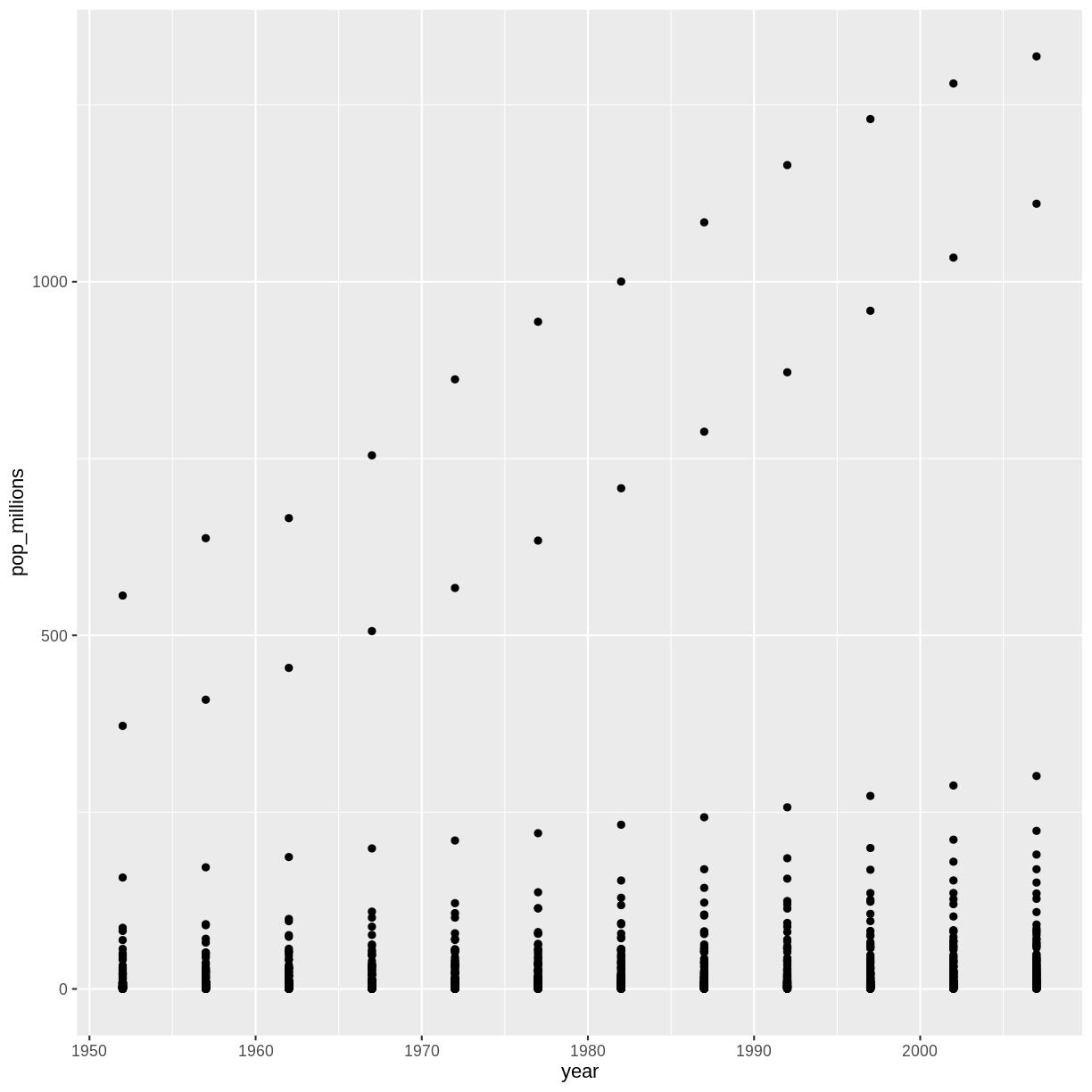
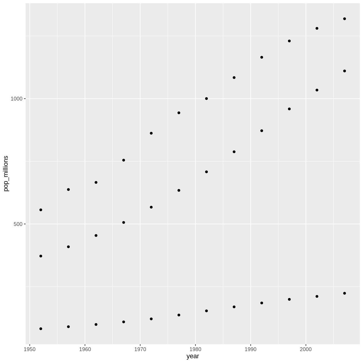
Comparison operators, logical operators, and many functions are also vectorized:
Comparison operators
x > 2
[1] FALSE FALSE TRUE TRUE
Logical operators
a <- x > 3 # or, for clarity, a <- (x > 3)
a
[1] FALSE FALSE FALSE TRUE
Tip: some useful functions for logical vectors
any()will returnTRUEif any element of a vector isTRUE.
all()will returnTRUEif all elements of a vector areTRUE.
Most functions also operate element-wise on vectors:
Functions
x <- 1:4
log(x)
[1] 0.0000000 0.6931472 1.0986123 1.3862944
Vectorized operations work element-wise on matrices:
m <- matrix(1:12, nrow=3, ncol=4)
m * -1
[,1] [,2] [,3] [,4]
[1,] -1 -4 -7 -10
[2,] -2 -5 -8 -11
[3,] -3 -6 -9 -12
Tip: element-wise vs. matrix multiplication
Very important: the operator
*gives you element-wise multiplication! To do matrix multiplication, we need to use the%*%operator:m %*% matrix(1, nrow=4, ncol=1)[,1] [1,] 22 [2,] 26 [3,] 30matrix(1:4, nrow=1) %*% matrix(1:4, ncol=1)[,1] [1,] 30For more on matrix algebra, see the Quick-R reference guide
Challenge 3
Given the following matrix:
m <- matrix(1:12, nrow=3, ncol=4) m[,1] [,2] [,3] [,4] [1,] 1 4 7 10 [2,] 2 5 8 11 [3,] 3 6 9 12Write down what you think will happen when you run:
m ^ -1m * c(1, 0, -1)m > c(0, 20)m * c(1, 0, -1, 2)Did you get the output you expected? If not, ask a helper!
Solution to challenge 3
Given the following matrix:
m <- matrix(1:12, nrow=3, ncol=4) m[,1] [,2] [,3] [,4] [1,] 1 4 7 10 [2,] 2 5 8 11 [3,] 3 6 9 12Write down what you think will happen when you run:
m ^ -1[,1] [,2] [,3] [,4] [1,] 1.0000000 0.2500000 0.1428571 0.10000000 [2,] 0.5000000 0.2000000 0.1250000 0.09090909 [3,] 0.3333333 0.1666667 0.1111111 0.08333333
m * c(1, 0, -1)[,1] [,2] [,3] [,4] [1,] 1 4 7 10 [2,] 0 0 0 0 [3,] -3 -6 -9 -12
m > c(0, 20)[,1] [,2] [,3] [,4] [1,] TRUE FALSE TRUE FALSE [2,] FALSE TRUE FALSE TRUE [3,] TRUE FALSE TRUE FALSE
Challenge 4
We’re interested in looking at the sum of the following sequence of fractions:
x = 1/(1^2) + 1/(2^2) + 1/(3^2) + ... + 1/(n^2)This would be tedious to type out, and impossible for high values of n. Use vectorisation to compute x when n=100. What is the sum when n=10,000?
Challenge 4
We’re interested in looking at the sum of the following sequence of fractions:
x = 1/(1^2) + 1/(2^2) + 1/(3^2) + ... + 1/(n^2)This would be tedious to type out, and impossible for high values of n. Can you use vectorisation to compute x, when n=100? How about when n=10,000?
sum(1/(1:100)^2)[1] 1.634984sum(1/(1:1e04)^2)[1] 1.644834n <- 10000 sum(1/(1:n)^2)[1] 1.644834We can also obtain the same results using a function:
inverse_sum_of_squares <- function(n) { sum(1/(1:n)^2) } inverse_sum_of_squares(100)[1] 1.634984inverse_sum_of_squares(10000)[1] 1.644834n <- 10000 inverse_sum_of_squares(n)[1] 1.644834
Key Points
Use vectorized operations instead of loops.
Functions Explained (extra)
Overview
Teaching: 0 min
Exercises: 0 minQuestions
How can I write a new function in R?
Objectives
Define a function that takes arguments.
Return a value from a function.
Check argument conditions with
stopifnot()in functions.Test a function.
Set default values for function arguments.
Explain why we should divide programs into small, single-purpose functions.
If we only had one data set to analyze, it would probably be faster to load the file into a spreadsheet and use that to plot simple statistics. However, the gapminder data is updated periodically, and we may want to pull in that new information later and re-run our analysis again. We may also obtain similar data from a different source in the future.
In this lesson, we’ll learn how to write a function so that we can repeat several operations with a single command.
What is a function?
Functions gather a sequence of operations into a whole, preserving it for ongoing use. Functions provide:
- a name we can remember and invoke it by
- relief from the need to remember the individual operations
- a defined set of inputs and expected outputs
- rich connections to the larger programming environment
As the basic building block of most programming languages, user-defined functions constitute “programming” as much as any single abstraction can. If you have written a function, you are a computer programmer.
Defining a function
Let’s open a new R script file in the functions/ directory and call it
functions-lesson.R.
The general structure of a function is:
my_function <- function(parameters) {
# perform action
# return value
}
Let’s define a function fahr_to_kelvin() that converts temperatures from
Fahrenheit to Kelvin:
fahr_to_kelvin <- function(temp) {
kelvin <- ((temp - 32) * (5 / 9)) + 273.15
return(kelvin)
}
We define fahr_to_kelvin() by assigning it to the output of function. The
list of argument names are contained within parentheses. Next, the
body of the function–the
statements that are executed when it runs–is contained within curly braces
({}). The statements in the body are indented by two spaces. This makes the
code easier to read but does not affect how the code operates.
It is useful to think of creating functions like writing a cookbook. First you define the “ingredients” that your function needs. In this case, we only need one ingredient to use our function: “temp”. After we list our ingredients, we then say what we will do with them, in this case, we are taking our ingredient and applying a set of mathematical operators to it.
When we call the function, the values we pass to it as arguments are assigned to those variables so that we can use them inside the function. Inside the function, we use a return statement to send a result back to whoever asked for it.
Tip
One feature unique to R is that the return statement is not required. R automatically returns whichever variable is on the last line of the body of the function. But for clarity, we will explicitly define the return statement.
Let’s try running our function. Calling our own function is no different from calling any other function:
# freezing point of water
fahr_to_kelvin(32)
[1] 273.15
# boiling point of water
fahr_to_kelvin(212)
[1] 373.15
Challenge 1
Write a function called
kelvin_to_celsius()that takes a temperature in Kelvin and returns that temperature in Celsius.Hint: To convert from Kelvin to Celsius you subtract 273.15
Solution to challenge 1
Write a function called
kelvin_to_celsiusthat takes a temperature in Kelvin and returns that temperature in Celsiuskelvin_to_celsius <- function(temp) { celsius <- temp - 273.15 return(celsius) }
Combining functions
The real power of functions comes from mixing, matching and combining them into ever-larger chunks to get the effect we want.
Let’s define two functions that will convert temperature from Fahrenheit to Kelvin, and Kelvin to Celsius:
fahr_to_kelvin <- function(temp) {
kelvin <- ((temp - 32) * (5 / 9)) + 273.15
return(kelvin)
}
kelvin_to_celsius <- function(temp) {
celsius <- temp - 273.15
return(celsius)
}
Challenge 2
Define the function to convert directly from Fahrenheit to Celsius, by reusing the two functions above (or using your own functions if you prefer).
Solution to challenge 2
Define the function to convert directly from Fahrenheit to Celsius, by reusing these two functions above
fahr_to_celsius <- function(temp) { temp_k <- fahr_to_kelvin(temp) result <- kelvin_to_celsius(temp_k) return(result) }
Interlude: Defensive Programming
Now that we’ve begun to appreciate how writing functions provides an efficient
way to make R code re-usable and modular, we should note that it is important
to ensure that functions only work in their intended use-cases. Checking
function parameters is related to the concept of defensive programming.
Defensive programming encourages us to frequently check conditions and throw an
error if something is wrong. These checks are referred to as assertion
statements because we want to assert some condition is TRUE before proceeding.
They make it easier to debug because they give us a better idea of where the
errors originate.
Checking conditions with stopifnot()
Let’s start by re-examining fahr_to_kelvin(), our function for converting
temperatures from Fahrenheit to Kelvin. It was defined like so:
fahr_to_kelvin <- function(temp) {
kelvin <- ((temp - 32) * (5 / 9)) + 273.15
return(kelvin)
}
For this function to work as intended, the argument temp must be a numeric
value; otherwise, the mathematical procedure for converting between the two
temperature scales will not work. To create an error, we can use the function
stop(). For example, since the argument temp must be a numeric vector, we
could check for this condition with an if statement and throw an error if the
condition was violated. We could augment our function above like so:
fahr_to_kelvin <- function(temp) {
if (!is.numeric(temp)) {
stop("temp must be a numeric vector.")
}
kelvin <- ((temp - 32) * (5 / 9)) + 273.15
return(kelvin)
}
If we had multiple conditions or arguments to check, it would take many lines
of code to check all of them. Luckily R provides the convenience function
stopifnot(). We can list as many requirements that should evaluate to TRUE;
stopifnot() throws an error if it finds one that is FALSE. Listing these
conditions also serves a secondary purpose as extra documentation for the
function.
Let’s try out defensive programming with stopifnot() by adding assertions to
check the input to our function fahr_to_kelvin().
We want to assert the following: temp is a numeric vector. We may do that like
so:
fahr_to_kelvin <- function(temp) {
stopifnot(is.numeric(temp))
kelvin <- ((temp - 32) * (5 / 9)) + 273.15
return(kelvin)
}
It still works when given proper input.
# freezing point of water
fahr_to_kelvin(temp = 32)
[1] 273.15
But fails instantly if given improper input.
# Metric is a factor instead of numeric
fahr_to_kelvin(temp = as.factor(32))
Error in fahr_to_kelvin(temp = as.factor(32)): is.numeric(temp) is not TRUE
Challenge 3
Use defensive programming to ensure that our
fahr_to_celsius()function throws an error immediately if the argumenttempis specified inappropriately.Solution to challenge 3
Extend our previous definition of the function by adding in an explicit call to
stopifnot(). Sincefahr_to_celsius()is a composition of two other functions, checking inside here makes adding checks to the two component functions redundant.fahr_to_celsius <- function(temp) { stopifnot(is.numeric(temp)) temp_k <- fahr_to_kelvin(temp) result <- kelvin_to_celsius(temp_k) return(result) }
More on combining functions
Now, we’re going to define a function that calculates the Gross Domestic Product of a nation from the data available in our dataset:
# Takes a dataset and multiplies the population column
# with the GDP per capita column.
calcGDP <- function(dat) {
gdp <- dat$pop * dat$gdpPercap
return(gdp)
}
We define calcGDP() by assigning it to the output of function. The list of
argument names are contained within parentheses. Next, the body of the function
– the statements executed when you call the function – is contained within
curly braces ({}).
We’ve indented the statements in the body by two spaces. This makes the code easier to read but does not affect how it operates.
When we call the function, the values we pass to it are assigned to the arguments, which become variables inside the body of the function.
Inside the function, we use the return() function to send back the result.
This return() function is optional: R will automatically return the results of
whatever command is executed on the last line of the function.
calcGDP(head(gapminder))
[1] 6567086330 7585448670 8758855797 9648014150 9678553274 11697659231
That’s not very informative. Let’s add some more arguments so we can extract that per year and country.
# Takes a dataset and multiplies the population column
# with the GDP per capita column.
calcGDP <- function(dat, year=NULL, country=NULL) {
if(!is.null(year)) {
dat <- dat[dat$year %in% year, ]
}
if (!is.null(country)) {
dat <- dat[dat$country %in% country,]
}
gdp <- dat$pop * dat$gdpPercap
new <- cbind(dat, gdp=gdp)
return(new)
}
If you’ve been writing these functions down into a separate R script
(a good idea!), you can load in the functions into our R session by using the
source() function:
source("functions/functions-lesson.R")
Ok, so there’s a lot going on in this function now. In plain English, the function now subsets the provided data by year if the year argument isn’t empty, then subsets the result by country if the country argument isn’t empty. Then it calculates the GDP for whatever subset emerges from the previous two steps. The function then adds the GDP as a new column to the subsetted data and returns this as the final result. You can see that the output is much more informative than a vector of numbers.
Let’s take a look at what happens when we specify the year:
head(calcGDP(gapminder, year=2007))
country year pop continent lifeExp gdpPercap gdp
12 Afghanistan 2007 31889923 Asia 43.828 974.5803 31079291949
24 Albania 2007 3600523 Europe 76.423 5937.0295 21376411360
36 Algeria 2007 33333216 Africa 72.301 6223.3675 207444851958
48 Angola 2007 12420476 Africa 42.731 4797.2313 59583895818
60 Argentina 2007 40301927 Americas 75.320 12779.3796 515033625357
72 Australia 2007 20434176 Oceania 81.235 34435.3674 703658358894
Or for a specific country:
calcGDP(gapminder, country="Australia")
country year pop continent lifeExp gdpPercap gdp
61 Australia 1952 8691212 Oceania 69.120 10039.60 87256254102
62 Australia 1957 9712569 Oceania 70.330 10949.65 106349227169
63 Australia 1962 10794968 Oceania 70.930 12217.23 131884573002
64 Australia 1967 11872264 Oceania 71.100 14526.12 172457986742
65 Australia 1972 13177000 Oceania 71.930 16788.63 221223770658
66 Australia 1977 14074100 Oceania 73.490 18334.20 258037329175
67 Australia 1982 15184200 Oceania 74.740 19477.01 295742804309
68 Australia 1987 16257249 Oceania 76.320 21888.89 355853119294
69 Australia 1992 17481977 Oceania 77.560 23424.77 409511234952
70 Australia 1997 18565243 Oceania 78.830 26997.94 501223252921
71 Australia 2002 19546792 Oceania 80.370 30687.75 599847158654
72 Australia 2007 20434176 Oceania 81.235 34435.37 703658358894
Or both:
calcGDP(gapminder, year=2007, country="Australia")
country year pop continent lifeExp gdpPercap gdp
72 Australia 2007 20434176 Oceania 81.235 34435.37 703658358894
Let’s walk through the body of the function:
calcGDP <- function(dat, year=NULL, country=NULL) {
Here we’ve added two arguments, year, and country. We’ve set
default arguments for both as NULL using the = operator
in the function definition. This means that those arguments will
take on those values unless the user specifies otherwise.
if(!is.null(year)) {
dat <- dat[dat$year %in% year, ]
}
if (!is.null(country)) {
dat <- dat[dat$country %in% country,]
}
Here, we check whether each additional argument is set to null, and whenever
they’re not null overwrite the dataset stored in dat with a subset given by
the non-null argument.
Building these conditionals into the function makes it more flexible for later. Now, we can use it to calculate the GDP for:
- The whole dataset;
- A single year;
- A single country;
- A single combination of year and country.
By using %in% instead, we can also give multiple years or countries to those
arguments.
Tip: Pass by value
Functions in R almost always make copies of the data to operate on inside of a function body. When we modify
datinside the function we are modifying the copy of the gapminder dataset stored indat, not the original variable we gave as the first argument.This is called “pass-by-value” and it makes writing code much safer: you can always be sure that whatever changes you make within the body of the function, stay inside the body of the function.
Tip: Function scope
Another important concept is scoping: any variables (or functions!) you create or modify inside the body of a function only exist for the lifetime of the function’s execution. When we call
calcGDP(), the variablesdat,gdpandnewonly exist inside the body of the function. Even if we have variables of the same name in our interactive R session, they are not modified in any way when executing a function.
gdp <- dat$pop * dat$gdpPercap
new <- cbind(dat, gdp=gdp)
return(new)
}
Finally, we calculated the GDP on our new subset, and created a new data frame with that column added. This means when we call the function later we can see the context for the returned GDP values, which is much better than in our first attempt where we got a vector of numbers.
Challenge 4
Test out your GDP function by calculating the GDP for New Zealand in 1987. How does this differ from New Zealand’s GDP in 1952?
Solution to challenge 4
calcGDP(gapminder, year = c(1952, 1987), country = "New Zealand")GDP for New Zealand in 1987: 65050008703
GDP for New Zealand in 1952: 21058193787
Challenge 5
The
paste()function can be used to combine text together, e.g:best_practice <- c("Write", "programs", "for", "people", "not", "computers") paste(best_practice, collapse=" ")[1] "Write programs for people not computers"Write a function called
fence()that takes two vectors as arguments, calledtextandwrapper, and prints out the text wrapped with thewrapper:fence(text=best_practice, wrapper="***")Note: the
paste()function has an argument calledsep, which specifies the separator between text. The default is a space: “ “. The default forpaste0()is no space “”.Solution to challenge 5
Write a function called
fence()that takes two vectors as arguments, calledtextandwrapper, and prints out the text wrapped with thewrapper:fence <- function(text, wrapper){ text <- c(wrapper, text, wrapper) result <- paste(text, collapse = " ") return(result) } best_practice <- c("Write", "programs", "for", "people", "not", "computers") fence(text=best_practice, wrapper="***")[1] "*** Write programs for people not computers ***"
Tip
R has some unique aspects that can be exploited when performing more complicated operations. We will not be writing anything that requires knowledge of these more advanced concepts. In the future when you are comfortable writing functions in R, you can learn more by reading the R Language Manual or this chapter from Advanced R Programming by Hadley Wickham.
Tip: Testing and documenting
It’s important to both test functions and document them: Documentation helps you, and others, understand what the purpose of your function is, and how to use it, and its important to make sure that your function actually does what you think.
When you first start out, your workflow will probably look a lot like this:
- Write a function
- Comment parts of the function to document its behaviour
- Load in the source file
- Experiment with it in the console to make sure it behaves as you expect
- Make any necessary bug fixes
- Rinse and repeat.
Formal documentation for functions, written in separate
.Rdfiles, gets turned into the documentation you see in help files. The roxygen2 package allows R coders to write documentation alongside the function code and then process it into the appropriate.Rdfiles. You will want to switch to this more formal method of writing documentation when you start writing more complicated R projects. In fact, packages are, in essence, bundles of functions with this formal documentation. Loading your own functions throughsource("functions.R")is equivalent to loading someone else’s functions (or your own one day!) throughlibrary("package").Formal automated tests can be written using the testthat package.
Key Points
Use
functionto define a new function in R.Use parameters to pass values into functions.
Use
stopifnot()to flexibly check function arguments in R.Load functions into programs using
source().
Writing Data (extra)
Overview
Teaching: 0 min
Exercises: 0 minQuestions
How can I save plots and data created in R?
Objectives
To be able to write out plots and data from R.
Saving plots
You have already seen how to save the most recent plot you create in ggplot2,
using the command ggsave. As a refresher:
ggsave("My_most_recent_plot.pdf")
You can save a plot from within RStudio using the ‘Export’ button in the ‘Plot’ window. This will give you the option of saving as a .pdf or as .png, .jpg or other image formats.
Sometimes you will want to save plots without creating them in the ‘Plot’ window first. Perhaps you want to make a pdf document with multiple pages: each one a different plot, for example. Or perhaps you’re looping through multiple subsets of a file, plotting data from each subset, and you want to save each plot, but obviously can’t stop the loop to click ‘Export’ for each one.
In this case you can use a more flexible approach. The function
pdf creates a new pdf device. You can control the size and resolution
using the arguments to this function.
pdf("Life_Exp_vs_time.pdf", width=12, height=4)
ggplot(data=gapminder, aes(x=year, y=lifeExp, colour=country)) +
geom_line() +
theme(legend.position = "none")
# You then have to make sure to turn off the pdf device!
dev.off()
Open up this document and have a look.
Challenge 1
Rewrite your ‘pdf’ command to print a second page in the pdf, showing a facet plot (hint: use
facet_grid) of the same data with one panel per continent.Solution to challenge 1
pdf("Life_Exp_vs_time.pdf", width = 12, height = 4) p <- ggplot(data = gapminder, aes(x = year, y = lifeExp, colour = country)) + geom_line() + theme(legend.position = "none") p p + facet_grid(~continent) dev.off()
The commands jpeg, png etc. are used similarly to produce
documents in different formats.
Writing data
At some point, you’ll also want to write out data from R.
We can use the write.table function for this, which is
very similar to read.table from before.
Let’s create a data-cleaning script, for this analysis, we only want to focus on the gapminder data for Australia:
aust_subset <- gapminder[gapminder$country == "Australia",]
write.table(aust_subset,
file="cleaned-data/gapminder-aus.csv",
sep=","
)
Let’s switch back to the shell to take a look at the data to make sure it looks OK:
head cleaned-data/gapminder-aus.csv
"country","year","pop","continent","lifeExp","gdpPercap"
"61","Australia",1952,8691212,"Oceania",69.12,10039.59564
"62","Australia",1957,9712569,"Oceania",70.33,10949.64959
"63","Australia",1962,10794968,"Oceania",70.93,12217.22686
"64","Australia",1967,11872264,"Oceania",71.1,14526.12465
"65","Australia",1972,13177000,"Oceania",71.93,16788.62948
"66","Australia",1977,14074100,"Oceania",73.49,18334.19751
"67","Australia",1982,15184200,"Oceania",74.74,19477.00928
"68","Australia",1987,16257249,"Oceania",76.32,21888.88903
"69","Australia",1992,17481977,"Oceania",77.56,23424.76683
Hmm, that’s not quite what we wanted. Where did all these quotation marks come from? Also the row numbers are meaningless.
Let’s look at the help file to work out how to change this behaviour.
?write.table
By default R will wrap character vectors with quotation marks when writing out to file. It will also write out the row and column names.
Let’s fix this:
write.table(
gapminder[gapminder$country == "Australia",],
file="cleaned-data/gapminder-aus.csv",
sep=",", quote=FALSE, row.names=FALSE
)
Now lets look at the data again using our shell skills:
head cleaned-data/gapminder-aus.csv
country,year,pop,continent,lifeExp,gdpPercap
Australia,1952,8691212,Oceania,69.12,10039.59564
Australia,1957,9712569,Oceania,70.33,10949.64959
Australia,1962,10794968,Oceania,70.93,12217.22686
Australia,1967,11872264,Oceania,71.1,14526.12465
Australia,1972,13177000,Oceania,71.93,16788.62948
Australia,1977,14074100,Oceania,73.49,18334.19751
Australia,1982,15184200,Oceania,74.74,19477.00928
Australia,1987,16257249,Oceania,76.32,21888.88903
Australia,1992,17481977,Oceania,77.56,23424.76683
That looks better!
Challenge 2
Write a data-cleaning script file that subsets the gapminder data to include only data points collected since 1990.
Use this script to write out the new subset to a file in the
cleaned-data/directory.Solution to challenge 2
write.table( gapminder[gapminder$year > 1990, ], file = "cleaned-data/gapminder-after1990.csv", sep = ",", quote = FALSE, row.names = FALSE )
Key Points
Save plots from RStudio using the ‘Export’ button.
Use
write.tableto save tabular data.
Splitting and Combining Data Frames with plyr (extra)
Overview
Teaching: 30 min
Exercises: 30 minQuestions
How can I do different calculations on different sets of data?
Objectives
To be able to use the split-apply-combine strategy for data analysis.
Previously we looked at how you can use functions to simplify your code.
We defined the calcGDP function, which takes the gapminder dataset,
and multiplies the population and GDP per capita column. We also defined
additional arguments so we could filter by year and country:
# Takes a dataset and multiplies the population column
# with the GDP per capita column.
calcGDP <- function(dat, year=NULL, country=NULL) {
if(!is.null(year)) {
dat <- dat[dat$year %in% year, ]
}
if (!is.null(country)) {
dat <- dat[dat$country %in% country,]
}
gdp <- dat$pop * dat$gdpPercap
new <- cbind(dat, gdp=gdp)
return(new)
}
A common task you’ll encounter when working with data, is that you’ll want to run calculations on different groups within the data. In the above, we were calculating the GDP by multiplying two columns together. But what if we wanted to calculated the mean GDP per continent?
We could run calcGDP and then take the mean of each continent:
withGDP <- calcGDP(gapminder)
mean(withGDP[withGDP$continent == "Africa", "gdp"])
[1] 20904782844
mean(withGDP[withGDP$continent == "Americas", "gdp"])
[1] 379262350210
mean(withGDP[withGDP$continent == "Asia", "gdp"])
[1] 227233738153
But this isn’t very nice. Yes, by using a function, you have reduced a substantial amount of repetition. That is nice. But there is still repetition. Repeating yourself will cost you time, both now and later, and potentially introduce some nasty bugs.
We could write a new function that is flexible like calcGDP, but this
also takes a substantial amount of effort and testing to get right.
The abstract problem we’re encountering here is know as “split-apply-combine”:
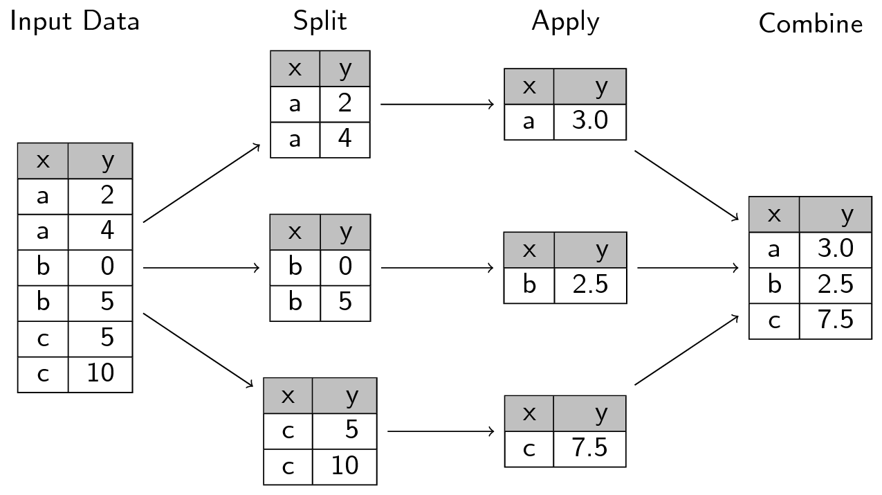
We want to split our data into groups, in this case continents, apply some calculations on that group, then optionally combine the results together afterwards.
The plyr package
For those of you who have used R before, you might be familiar with the
apply family of functions. While R’s built in functions do work, we’re
going to introduce you to another method for solving the “split-apply-combine”
problem. The plyr package provides a set of
functions that we find more user friendly for solving this problem.
We installed this package in an earlier challenge. Let us load it now:
library("plyr")
Plyr has functions for operating on lists, data.frames and arrays
(matrices, or n-dimensional vectors). Each function performs:
- A splitting operation
- Apply a function on each split in turn.
- Recombine output data as a single data object.
The functions are named based on the data structure they expect as input, and the data structure you want returned as output: [a]rray, [l]ist, or [d]ata.frame. The first letter corresponds to the input data structure, the second letter to the output data structure, and then the rest of the function is named “ply”.
This gives us 9 core functions **ply. There are an additional three functions
which will only perform the split and apply steps, and not any combine step.
They’re named by their input data type and represent null output by a _ (see
table)
Note here that plyr’s use of “array” is different to R’s, an array in ply can include a vector or matrix.
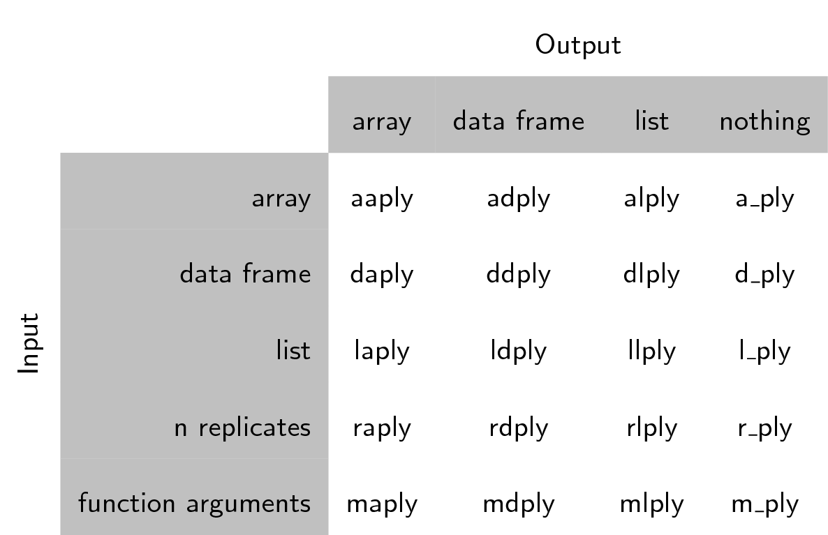
Each of the xxply functions (daply, ddply, llply, laply, …) has the
same structure and has 4 key features and structure:
xxply(.data, .variables, .fun)
- The first letter of the function name gives the input type and the second gives the output type.
- .data - gives the data object to be processed
- .variables - identifies the splitting variables
- .fun - gives the function to be called on each piece
Now we can quickly calculate the mean GDP per continent:
ddply(
.data = calcGDP(gapminder),
.variables = "continent",
.fun = function(x) mean(x$gdp)
)
continent V1
1 Africa 20904782844
2 Americas 379262350210
3 Asia 227233738153
4 Europe 269442085301
5 Oceania 188187105354
Let us walk through the previous code:
- The
ddplyfunction feeds in adata.frame(function starts with d) and returns anotherdata.frame(2nd letter is a d) - the first argument we gave was the data.frame we wanted to operate on: in this
case the gapminder data. We called
calcGDPon it first so that it would have the additionalgdpcolumn added to it. - The second argument indicated our split criteria: in this case the “continent” column. Note that we gave the name of the column, not the values of the column like we had done previously with subsetting. Plyr takes care of these implementation details for you.
- The third argument is the function we want to apply to each grouping of the
data. We had to define our own short function here: each subset of the data
gets stored in
x, the first argument of our function. This is an anonymous function: we haven’t defined it elsewhere, and it has no name. It only exists in the scope of our call toddply.
Challenge 1
Calculate the average life expectancy per continent. Which has the longest? Which had the shortest?
Solution to Challenge 1
ddply( .data = gapminder, .variables = "continent", .fun = function(x) mean(x$lifeExp) )Oceania has the longest and Africa the shortest.
What if we want a different type of output data structure?:
dlply(
.data = calcGDP(gapminder),
.variables = "continent",
.fun = function(x) mean(x$gdp)
)
$Africa
[1] 20904782844
$Americas
[1] 379262350210
$Asia
[1] 227233738153
$Europe
[1] 269442085301
$Oceania
[1] 188187105354
attr(,"split_type")
[1] "data.frame"
attr(,"split_labels")
continent
1 Africa
2 Americas
3 Asia
4 Europe
5 Oceania
We called the same function again, but changed the second letter to an l, so
the output was returned as a list.
We can specify multiple columns to group by:
ddply(
.data = calcGDP(gapminder),
.variables = c("continent", "year"),
.fun = function(x) mean(x$gdp)
)
continent year V1
1 Africa 1952 5992294608
2 Africa 1957 7359188796
3 Africa 1962 8784876958
4 Africa 1967 11443994101
5 Africa 1972 15072241974
6 Africa 1977 18694898732
7 Africa 1982 22040401045
8 Africa 1987 24107264108
9 Africa 1992 26256977719
10 Africa 1997 30023173824
11 Africa 2002 35303511424
12 Africa 2007 45778570846
13 Americas 1952 117738997171
14 Americas 1957 140817061264
15 Americas 1962 169153069442
16 Americas 1967 217867530844
17 Americas 1972 268159178814
18 Americas 1977 324085389022
19 Americas 1982 363314008350
20 Americas 1987 439447790357
21 Americas 1992 489899820623
22 Americas 1997 582693307146
23 Americas 2002 661248623419
24 Americas 2007 776723426068
25 Asia 1952 34095762661
26 Asia 1957 47267432088
27 Asia 1962 60136869012
28 Asia 1967 84648519224
29 Asia 1972 124385747313
30 Asia 1977 159802590186
31 Asia 1982 194429049919
32 Asia 1987 241784763369
33 Asia 1992 307100497486
34 Asia 1997 387597655323
35 Asia 2002 458042336179
36 Asia 2007 627513635079
37 Europe 1952 84971341466
38 Europe 1957 109989505140
39 Europe 1962 138984693095
40 Europe 1967 173366641137
41 Europe 1972 218691462733
42 Europe 1977 255367522034
43 Europe 1982 279484077072
44 Europe 1987 316507473546
45 Europe 1992 342703247405
46 Europe 1997 383606933833
47 Europe 2002 436448815097
48 Europe 2007 493183311052
49 Oceania 1952 54157223944
50 Oceania 1957 66826828013
51 Oceania 1962 82336453245
52 Oceania 1967 105958863585
53 Oceania 1972 134112109227
54 Oceania 1977 154707711162
55 Oceania 1982 176177151380
56 Oceania 1987 209451563998
57 Oceania 1992 236319179826
58 Oceania 1997 289304255183
59 Oceania 2002 345236880176
60 Oceania 2007 403657044512
daply(
.data = calcGDP(gapminder),
.variables = c("continent", "year"),
.fun = function(x) mean(x$gdp)
)
year
continent 1952 1957 1962 1967 1972
Africa 5992294608 7359188796 8784876958 11443994101 15072241974
Americas 117738997171 140817061264 169153069442 217867530844 268159178814
Asia 34095762661 47267432088 60136869012 84648519224 124385747313
Europe 84971341466 109989505140 138984693095 173366641137 218691462733
Oceania 54157223944 66826828013 82336453245 105958863585 134112109227
year
continent 1977 1982 1987 1992 1997
Africa 18694898732 22040401045 24107264108 26256977719 30023173824
Americas 324085389022 363314008350 439447790357 489899820623 582693307146
Asia 159802590186 194429049919 241784763369 307100497486 387597655323
Europe 255367522034 279484077072 316507473546 342703247405 383606933833
Oceania 154707711162 176177151380 209451563998 236319179826 289304255183
year
continent 2002 2007
Africa 35303511424 45778570846
Americas 661248623419 776723426068
Asia 458042336179 627513635079
Europe 436448815097 493183311052
Oceania 345236880176 403657044512
You can use these functions in place of for loops (and it is usually faster to
do so).
To replace a for loop, put the code that was in the body of the for loop inside an anonymous function.
d_ply(
.data=gapminder,
.variables = "continent",
.fun = function(x) {
meanGDPperCap <- mean(x$gdpPercap)
print(paste(
"The mean GDP per capita for", unique(x$continent),
"is", format(meanGDPperCap, big.mark=",")
))
}
)
[1] "The mean GDP per capita for Africa is 2,193.755"
[1] "The mean GDP per capita for Americas is 7,136.11"
[1] "The mean GDP per capita for Asia is 7,902.15"
[1] "The mean GDP per capita for Europe is 14,469.48"
[1] "The mean GDP per capita for Oceania is 18,621.61"
Tip: printing numbers
The
formatfunction can be used to make numeric values “pretty” for printing out in messages.
Challenge 2
Calculate the average life expectancy per continent and year. Which had the longest and shortest in 2007? Which had the greatest change in between 1952 and 2007?
Solution to Challenge 2
solution <- ddply( .data = gapminder, .variables = c("continent", "year"), .fun = function(x) mean(x$lifeExp) ) solution_2007 <- solution[solution$year == 2007, ] solution_2007Oceania had the longest average life expectancy in 2007 and Africa the lowest.
solution_1952_2007 <- cbind(solution[solution$year == 1952, ], solution_2007) difference_1952_2007 <- data.frame(continent = solution_1952_2007$continent, year_1957 = solution_1952_2007[[3]], year_2007 = solution_1952_2007[[6]], difference = solution_1952_2007[[6]] - solution_1952_2007[[3]]) difference_1952_2007Asia had the greatest difference, and Oceania the least.
Alternate Challenge
Without running them, which of the following will calculate the average life expectancy per continent:
1.
ddply( .data = gapminder, .variables = gapminder$continent, .fun = function(dataGroup) { mean(dataGroup$lifeExp) } )2.
ddply( .data = gapminder, .variables = "continent", .fun = mean(dataGroup$lifeExp) )3.
ddply( .data = gapminder, .variables = "continent", .fun = function(dataGroup) { mean(dataGroup$lifeExp) } )4.
adply( .data = gapminder, .variables = "continent", .fun = function(dataGroup) { mean(dataGroup$lifeExp) } )Solution to Alternative Challenge
Answer 3 will calculate the average life expectancy per continent.
Key Points
Use the
plyrpackage to split data, apply functions to subsets, and combine the results.
Data Frame Manipulation with tidyr (extra)
Overview
Teaching: 0 min
Exercises: 0 minQuestions
How can I change the layout of a data frame?
Objectives
To understand the concepts of ‘longer’ and ‘wider’ data frame formats and be able to convert between them with
tidyr.
Researchers often want to reshape their data frames from ‘wide’ to ‘longer’ layouts, or vice-versa. The ‘long’ layout or format is where:
- each column is a variable
- each row is an observation
In the purely ‘long’ (or ‘longest’) format, you usually have 1 column for the observed variable and the other columns are ID variables.
For the ‘wide’ format each row is often a site/subject/patient and you have
multiple observation variables containing the same type of data. These can be
either repeated observations over time, or observation of multiple variables (or
a mix of both). You may find data input may be simpler or some other
applications may prefer the ‘wide’ format. However, many of R’s functions have
been designed assuming you have ‘longer’ formatted data. This tutorial will help you
efficiently transform your data shape regardless of original format.
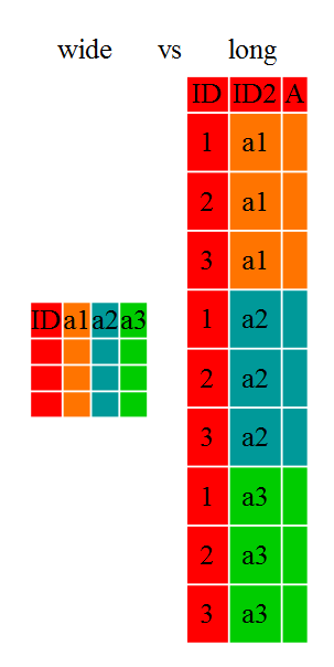
Long and wide data frame layouts mainly affect readability. For humans, the wide format is often more intuitive since we can often see more of the data on the screen due to its shape. However, the long format is more machine readable and is closer to the formatting of databases. The ID variables in our data frames are similar to the fields in a database and observed variables are like the database values.
Getting started
First install the packages if you haven’t already done so (you probably installed dplyr in the previous lesson):
#install.packages("tidyr")
#install.packages("dplyr")
Load the packages
library("tidyr")
library("dplyr")
First, lets look at the structure of our original gapminder data frame:
str(gapminder)
'data.frame': 1704 obs. of 6 variables:
$ country : chr "Afghanistan" "Afghanistan" "Afghanistan" "Afghanistan" ...
$ year : int 1952 1957 1962 1967 1972 1977 1982 1987 1992 1997 ...
$ pop : num 8425333 9240934 10267083 11537966 13079460 ...
$ continent: chr "Asia" "Asia" "Asia" "Asia" ...
$ lifeExp : num 28.8 30.3 32 34 36.1 ...
$ gdpPercap: num 779 821 853 836 740 ...
Challenge 1
Is gapminder a purely long, purely wide, or some intermediate format?
Solution to Challenge 1
The original gapminder data.frame is in an intermediate format. It is not purely long since it had multiple observation variables (
pop,lifeExp,gdpPercap).
Sometimes, as with the gapminder dataset, we have multiple types of observed
data. It is somewhere in between the purely ‘long’ and ‘wide’ data formats. We
have 3 “ID variables” (continent, country, year) and 3 “Observation
variables” (pop,lifeExp,gdpPercap). This intermediate format can be
preferred despite not having ALL observations in 1 column given that all 3
observation variables have different units. There are few operations that would
need us to make this data frame any longer (i.e. 4 ID variables and 1
Observation variable).
While using many of the functions in R, which are often vector based, you
usually do not want to do mathematical operations on values with different
units. For example, using the purely long format, a single mean for all of the
values of population, life expectancy, and GDP would not be meaningful since it
would return the mean of values with 3 incompatible units. The solution is that
we first manipulate the data either by grouping (see the lesson on dplyr), or
we change the structure of the data frame. Note: Some plotting functions in
R actually work better in the wide format data.
From wide to long format with pivot_longer()
Until now, we’ve been using the nicely formatted original gapminder dataset, but ‘real’ data (i.e. our own research data) will never be so well organized. Here let’s start with the wide formatted version of the gapminder dataset.
Download the wide version of the gapminder data from here and save it in your data folder.
We’ll load the data file and look at it. Note: we don’t want our continent and
country columns to be factors, so we use the stringsAsFactors argument for
read.csv() to disable that.
gap_wide <- read.csv("data/gapminder_wide.csv", stringsAsFactors = FALSE)
str(gap_wide)
'data.frame': 142 obs. of 38 variables:
$ continent : chr "Africa" "Africa" "Africa" "Africa" ...
$ country : chr "Algeria" "Angola" "Benin" "Botswana" ...
$ gdpPercap_1952: num 2449 3521 1063 851 543 ...
$ gdpPercap_1957: num 3014 3828 960 918 617 ...
$ gdpPercap_1962: num 2551 4269 949 984 723 ...
$ gdpPercap_1967: num 3247 5523 1036 1215 795 ...
$ gdpPercap_1972: num 4183 5473 1086 2264 855 ...
$ gdpPercap_1977: num 4910 3009 1029 3215 743 ...
$ gdpPercap_1982: num 5745 2757 1278 4551 807 ...
$ gdpPercap_1987: num 5681 2430 1226 6206 912 ...
$ gdpPercap_1992: num 5023 2628 1191 7954 932 ...
$ gdpPercap_1997: num 4797 2277 1233 8647 946 ...
$ gdpPercap_2002: num 5288 2773 1373 11004 1038 ...
$ gdpPercap_2007: num 6223 4797 1441 12570 1217 ...
$ lifeExp_1952 : num 43.1 30 38.2 47.6 32 ...
$ lifeExp_1957 : num 45.7 32 40.4 49.6 34.9 ...
$ lifeExp_1962 : num 48.3 34 42.6 51.5 37.8 ...
$ lifeExp_1967 : num 51.4 36 44.9 53.3 40.7 ...
$ lifeExp_1972 : num 54.5 37.9 47 56 43.6 ...
$ lifeExp_1977 : num 58 39.5 49.2 59.3 46.1 ...
$ lifeExp_1982 : num 61.4 39.9 50.9 61.5 48.1 ...
$ lifeExp_1987 : num 65.8 39.9 52.3 63.6 49.6 ...
$ lifeExp_1992 : num 67.7 40.6 53.9 62.7 50.3 ...
$ lifeExp_1997 : num 69.2 41 54.8 52.6 50.3 ...
$ lifeExp_2002 : num 71 41 54.4 46.6 50.6 ...
$ lifeExp_2007 : num 72.3 42.7 56.7 50.7 52.3 ...
$ pop_1952 : num 9279525 4232095 1738315 442308 4469979 ...
$ pop_1957 : num 10270856 4561361 1925173 474639 4713416 ...
$ pop_1962 : num 11000948 4826015 2151895 512764 4919632 ...
$ pop_1967 : num 12760499 5247469 2427334 553541 5127935 ...
$ pop_1972 : num 14760787 5894858 2761407 619351 5433886 ...
$ pop_1977 : num 17152804 6162675 3168267 781472 5889574 ...
$ pop_1982 : num 20033753 7016384 3641603 970347 6634596 ...
$ pop_1987 : num 23254956 7874230 4243788 1151184 7586551 ...
$ pop_1992 : num 26298373 8735988 4981671 1342614 8878303 ...
$ pop_1997 : num 29072015 9875024 6066080 1536536 10352843 ...
$ pop_2002 : int 31287142 10866106 7026113 1630347 12251209 7021078 15929988 4048013 8835739 614382 ...
$ pop_2007 : int 33333216 12420476 8078314 1639131 14326203 8390505 17696293 4369038 10238807 710960 ...
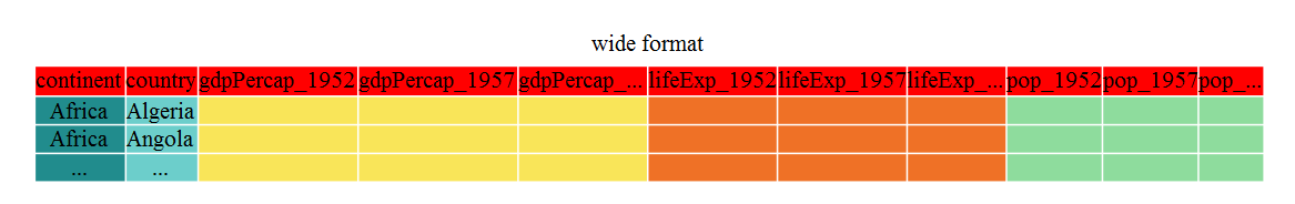
To change this very wide data frame layout back to our nice, intermediate (or longer) layout, we will use one of the two available pivot functions from the tidyr package. To convert from wide to a longer format, we will use the pivot_longer() function. pivot_longer() makes datasets longer by increasing the number of rows and decreasing the number of columns, or ‘lengthening’ your observation variables into a single variable.
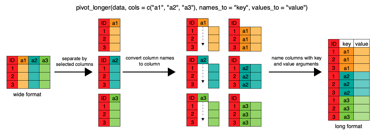
gap_long <- gap_wide %>%
pivot_longer(
cols = c(starts_with('pop'), starts_with('lifeExp'), starts_with('gdpPercap')),
names_to = "obstype_year", values_to = "obs_values"
)
str(gap_long)
tibble [5,112 × 4] (S3: tbl_df/tbl/data.frame)
$ continent : chr [1:5112] "Africa" "Africa" "Africa" "Africa" ...
$ country : chr [1:5112] "Algeria" "Algeria" "Algeria" "Algeria" ...
$ obstype_year: chr [1:5112] "pop_1952" "pop_1957" "pop_1962" "pop_1967" ...
$ obs_values : num [1:5112] 9279525 10270856 11000948 12760499 14760787 ...
Here we have used piping syntax which is similar to what we were doing in the previous lesson with dplyr. In fact, these are compatible and you can use a mix of tidyr and dplyr functions by piping them together.
We first provide to pivot_longer() a vector of column names that will be
pivoted into longer format. We could type out all the observation variables, but
as in the select() function (see dplyr lesson), we can use the starts_with()
argument to select all variables that start with the desired character string.
pivot_longer() also allows the alternative syntax of using the - symbol to
identify which variables are not to be pivoted (i.e. ID variables).
The next arguments to pivot_longer() are names_to for naming the column that
will contain the new ID variable (obstype_year) and values_to for naming the
new amalgamated observation variable (obs_value). We supply these new column
names as strings.
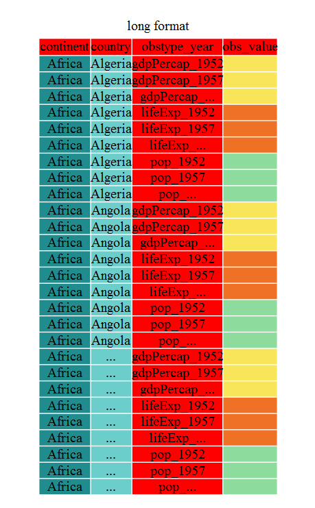
gap_long <- gap_wide %>%
pivot_longer(
cols = c(-continent, -country),
names_to = "obstype_year", values_to = "obs_values"
)
str(gap_long)
tibble [5,112 × 4] (S3: tbl_df/tbl/data.frame)
$ continent : chr [1:5112] "Africa" "Africa" "Africa" "Africa" ...
$ country : chr [1:5112] "Algeria" "Algeria" "Algeria" "Algeria" ...
$ obstype_year: chr [1:5112] "gdpPercap_1952" "gdpPercap_1957" "gdpPercap_1962" "gdpPercap_1967" ...
$ obs_values : num [1:5112] 2449 3014 2551 3247 4183 ...
That may seem trivial with this particular data frame, but sometimes you have 1 ID variable and 40 observation variables with irregular variable names. The flexibility is a huge time saver!
Now obstype_year actually contains 2 pieces of information, the observation
type (pop,lifeExp, or gdpPercap) and the year. We can use the
separate() function to split the character strings into multiple variables
gap_long <- gap_long %>% separate(obstype_year, into = c('obs_type', 'year'), sep = "_")
gap_long$year <- as.integer(gap_long$year)
Challenge 2
Using
gap_long, calculate the mean life expectancy, population, and gdpPercap for each continent. Hint: use thegroup_by()andsummarize()functions we learned in thedplyrlessonSolution to Challenge 2
gap_long %>% group_by(continent, obs_type) %>% summarize(means=mean(obs_values))`summarise()` has grouped output by 'continent'. You can override using the `.groups` argument.# A tibble: 15 × 3 # Groups: continent [5] continent obs_type means <chr> <chr> <dbl> 1 Africa gdpPercap 2194. 2 Africa lifeExp 48.9 3 Africa pop 9916003. 4 Americas gdpPercap 7136. 5 Americas lifeExp 64.7 6 Americas pop 24504795. 7 Asia gdpPercap 7902. 8 Asia lifeExp 60.1 9 Asia pop 77038722. 10 Europe gdpPercap 14469. 11 Europe lifeExp 71.9 12 Europe pop 17169765. 13 Oceania gdpPercap 18622. 14 Oceania lifeExp 74.3 15 Oceania pop 8874672.
From long to intermediate format with pivot_wider()
It is always good to check work. So, let’s use the second pivot function, pivot_wider(), to ‘widen’ our observation variables back out. pivot_wider() is the opposite of pivot_longer(), making a dataset wider by increasing the number of columns and decreasing the number of rows. We can use pivot_wider() to pivot or reshape our gap_long to the original intermediate format or the widest format. Let’s start with the intermediate format.
The pivot_wider() function takes names_from and values_from arguments.
To names_from we supply the column name whose contents will be pivoted into new
output columns in the widened data frame. The corresponding values will be added
from the column named in the values_from argument.
gap_normal <- gap_long %>%
pivot_wider(names_from = obs_type, values_from = obs_values)
dim(gap_normal)
[1] 1704 6
dim(gapminder)
[1] 1704 6
names(gap_normal)
[1] "continent" "country" "year" "gdpPercap" "lifeExp" "pop"
names(gapminder)
[1] "country" "year" "pop" "continent" "lifeExp" "gdpPercap"
Now we’ve got an intermediate data frame gap_normal with the same dimensions as
the original gapminder, but the order of the variables is different. Let’s fix
that before checking if they are all.equal().
gap_normal <- gap_normal[, names(gapminder)]
all.equal(gap_normal, gapminder)
[1] "Attributes: < Component \"class\": Lengths (3, 1) differ (string compare on first 1) >"
[2] "Attributes: < Component \"class\": 1 string mismatch >"
[3] "Component \"country\": 1704 string mismatches"
[4] "Component \"pop\": Mean relative difference: 1.634504"
[5] "Component \"continent\": 1212 string mismatches"
[6] "Component \"lifeExp\": Mean relative difference: 0.203822"
[7] "Component \"gdpPercap\": Mean relative difference: 1.162302"
head(gap_normal)
# A tibble: 6 × 6
country year pop continent lifeExp gdpPercap
<chr> <int> <dbl> <chr> <dbl> <dbl>
1 Algeria 1952 9279525 Africa 43.1 2449.
2 Algeria 1957 10270856 Africa 45.7 3014.
3 Algeria 1962 11000948 Africa 48.3 2551.
4 Algeria 1967 12760499 Africa 51.4 3247.
5 Algeria 1972 14760787 Africa 54.5 4183.
6 Algeria 1977 17152804 Africa 58.0 4910.
head(gapminder)
country year pop continent lifeExp gdpPercap
1 Afghanistan 1952 8425333 Asia 28.801 779.4453
2 Afghanistan 1957 9240934 Asia 30.332 820.8530
3 Afghanistan 1962 10267083 Asia 31.997 853.1007
4 Afghanistan 1967 11537966 Asia 34.020 836.1971
5 Afghanistan 1972 13079460 Asia 36.088 739.9811
6 Afghanistan 1977 14880372 Asia 38.438 786.1134
We’re almost there, the original was sorted by country, then
year.
gap_normal <- gap_normal %>% arrange(country, year)
all.equal(gap_normal, gapminder)
[1] "Attributes: < Component \"class\": Lengths (3, 1) differ (string compare on first 1) >"
[2] "Attributes: < Component \"class\": 1 string mismatch >"
That’s great! We’ve gone from the longest format back to the intermediate and we didn’t introduce any errors in our code.
Now let’s convert the long all the way back to the wide. In the wide format, we
will keep country and continent as ID variables and pivot the observations
across the 3 metrics (pop,lifeExp,gdpPercap) and time (year). First we
need to create appropriate labels for all our new variables (time*metric
combinations) and we also need to unify our ID variables to simplify the process
of defining gap_wide.
gap_temp <- gap_long %>% unite(var_ID, continent, country, sep = "_")
str(gap_temp)
tibble [5,112 × 4] (S3: tbl_df/tbl/data.frame)
$ var_ID : chr [1:5112] "Africa_Algeria" "Africa_Algeria" "Africa_Algeria" "Africa_Algeria" ...
$ obs_type : chr [1:5112] "gdpPercap" "gdpPercap" "gdpPercap" "gdpPercap" ...
$ year : int [1:5112] 1952 1957 1962 1967 1972 1977 1982 1987 1992 1997 ...
$ obs_values: num [1:5112] 2449 3014 2551 3247 4183 ...
gap_temp <- gap_long %>%
unite(ID_var, continent, country, sep = "_") %>%
unite(var_names, obs_type, year, sep = "_")
str(gap_temp)
tibble [5,112 × 3] (S3: tbl_df/tbl/data.frame)
$ ID_var : chr [1:5112] "Africa_Algeria" "Africa_Algeria" "Africa_Algeria" "Africa_Algeria" ...
$ var_names : chr [1:5112] "gdpPercap_1952" "gdpPercap_1957" "gdpPercap_1962" "gdpPercap_1967" ...
$ obs_values: num [1:5112] 2449 3014 2551 3247 4183 ...
Using unite() we now have a single ID variable which is a combination of
continent,country,and we have defined variable names. We’re now ready to
pipe in pivot_wider()
gap_wide_new <- gap_long %>%
unite(ID_var, continent, country, sep = "_") %>%
unite(var_names, obs_type, year, sep = "_") %>%
pivot_wider(names_from = var_names, values_from = obs_values)
str(gap_wide_new)
tibble [142 × 37] (S3: tbl_df/tbl/data.frame)
$ ID_var : chr [1:142] "Africa_Algeria" "Africa_Angola" "Africa_Benin" "Africa_Botswana" ...
$ gdpPercap_1952: num [1:142] 2449 3521 1063 851 543 ...
$ gdpPercap_1957: num [1:142] 3014 3828 960 918 617 ...
$ gdpPercap_1962: num [1:142] 2551 4269 949 984 723 ...
$ gdpPercap_1967: num [1:142] 3247 5523 1036 1215 795 ...
$ gdpPercap_1972: num [1:142] 4183 5473 1086 2264 855 ...
$ gdpPercap_1977: num [1:142] 4910 3009 1029 3215 743 ...
$ gdpPercap_1982: num [1:142] 5745 2757 1278 4551 807 ...
$ gdpPercap_1987: num [1:142] 5681 2430 1226 6206 912 ...
$ gdpPercap_1992: num [1:142] 5023 2628 1191 7954 932 ...
$ gdpPercap_1997: num [1:142] 4797 2277 1233 8647 946 ...
$ gdpPercap_2002: num [1:142] 5288 2773 1373 11004 1038 ...
$ gdpPercap_2007: num [1:142] 6223 4797 1441 12570 1217 ...
$ lifeExp_1952 : num [1:142] 43.1 30 38.2 47.6 32 ...
$ lifeExp_1957 : num [1:142] 45.7 32 40.4 49.6 34.9 ...
$ lifeExp_1962 : num [1:142] 48.3 34 42.6 51.5 37.8 ...
$ lifeExp_1967 : num [1:142] 51.4 36 44.9 53.3 40.7 ...
$ lifeExp_1972 : num [1:142] 54.5 37.9 47 56 43.6 ...
$ lifeExp_1977 : num [1:142] 58 39.5 49.2 59.3 46.1 ...
$ lifeExp_1982 : num [1:142] 61.4 39.9 50.9 61.5 48.1 ...
$ lifeExp_1987 : num [1:142] 65.8 39.9 52.3 63.6 49.6 ...
$ lifeExp_1992 : num [1:142] 67.7 40.6 53.9 62.7 50.3 ...
$ lifeExp_1997 : num [1:142] 69.2 41 54.8 52.6 50.3 ...
$ lifeExp_2002 : num [1:142] 71 41 54.4 46.6 50.6 ...
$ lifeExp_2007 : num [1:142] 72.3 42.7 56.7 50.7 52.3 ...
$ pop_1952 : num [1:142] 9279525 4232095 1738315 442308 4469979 ...
$ pop_1957 : num [1:142] 10270856 4561361 1925173 474639 4713416 ...
$ pop_1962 : num [1:142] 11000948 4826015 2151895 512764 4919632 ...
$ pop_1967 : num [1:142] 12760499 5247469 2427334 553541 5127935 ...
$ pop_1972 : num [1:142] 14760787 5894858 2761407 619351 5433886 ...
$ pop_1977 : num [1:142] 17152804 6162675 3168267 781472 5889574 ...
$ pop_1982 : num [1:142] 20033753 7016384 3641603 970347 6634596 ...
$ pop_1987 : num [1:142] 23254956 7874230 4243788 1151184 7586551 ...
$ pop_1992 : num [1:142] 26298373 8735988 4981671 1342614 8878303 ...
$ pop_1997 : num [1:142] 29072015 9875024 6066080 1536536 10352843 ...
$ pop_2002 : num [1:142] 31287142 10866106 7026113 1630347 12251209 ...
$ pop_2007 : num [1:142] 33333216 12420476 8078314 1639131 14326203 ...
Challenge 3
Take this 1 step further and create a
gap_ludicrously_wideformat data by pivoting over countries, year and the 3 metrics? Hint this new data frame should only have 5 rows.Solution to Challenge 3
gap_ludicrously_wide <- gap_long %>% unite(var_names, obs_type, year, country, sep = "_") %>% pivot_wider(names_from = var_names, values_from = obs_values)
Now we have a great ‘wide’ format data frame, but the ID_var could be more
usable, let’s separate it into 2 variables with separate()
gap_wide_betterID <- separate(gap_wide_new, ID_var, c("continent", "country"), sep="_")
gap_wide_betterID <- gap_long %>%
unite(ID_var, continent, country, sep = "_") %>%
unite(var_names, obs_type, year, sep = "_") %>%
pivot_wider(names_from = var_names, values_from = obs_values) %>%
separate(ID_var, c("continent","country"), sep = "_")
str(gap_wide_betterID)
tibble [142 × 38] (S3: tbl_df/tbl/data.frame)
$ continent : chr [1:142] "Africa" "Africa" "Africa" "Africa" ...
$ country : chr [1:142] "Algeria" "Angola" "Benin" "Botswana" ...
$ gdpPercap_1952: num [1:142] 2449 3521 1063 851 543 ...
$ gdpPercap_1957: num [1:142] 3014 3828 960 918 617 ...
$ gdpPercap_1962: num [1:142] 2551 4269 949 984 723 ...
$ gdpPercap_1967: num [1:142] 3247 5523 1036 1215 795 ...
$ gdpPercap_1972: num [1:142] 4183 5473 1086 2264 855 ...
$ gdpPercap_1977: num [1:142] 4910 3009 1029 3215 743 ...
$ gdpPercap_1982: num [1:142] 5745 2757 1278 4551 807 ...
$ gdpPercap_1987: num [1:142] 5681 2430 1226 6206 912 ...
$ gdpPercap_1992: num [1:142] 5023 2628 1191 7954 932 ...
$ gdpPercap_1997: num [1:142] 4797 2277 1233 8647 946 ...
$ gdpPercap_2002: num [1:142] 5288 2773 1373 11004 1038 ...
$ gdpPercap_2007: num [1:142] 6223 4797 1441 12570 1217 ...
$ lifeExp_1952 : num [1:142] 43.1 30 38.2 47.6 32 ...
$ lifeExp_1957 : num [1:142] 45.7 32 40.4 49.6 34.9 ...
$ lifeExp_1962 : num [1:142] 48.3 34 42.6 51.5 37.8 ...
$ lifeExp_1967 : num [1:142] 51.4 36 44.9 53.3 40.7 ...
$ lifeExp_1972 : num [1:142] 54.5 37.9 47 56 43.6 ...
$ lifeExp_1977 : num [1:142] 58 39.5 49.2 59.3 46.1 ...
$ lifeExp_1982 : num [1:142] 61.4 39.9 50.9 61.5 48.1 ...
$ lifeExp_1987 : num [1:142] 65.8 39.9 52.3 63.6 49.6 ...
$ lifeExp_1992 : num [1:142] 67.7 40.6 53.9 62.7 50.3 ...
$ lifeExp_1997 : num [1:142] 69.2 41 54.8 52.6 50.3 ...
$ lifeExp_2002 : num [1:142] 71 41 54.4 46.6 50.6 ...
$ lifeExp_2007 : num [1:142] 72.3 42.7 56.7 50.7 52.3 ...
$ pop_1952 : num [1:142] 9279525 4232095 1738315 442308 4469979 ...
$ pop_1957 : num [1:142] 10270856 4561361 1925173 474639 4713416 ...
$ pop_1962 : num [1:142] 11000948 4826015 2151895 512764 4919632 ...
$ pop_1967 : num [1:142] 12760499 5247469 2427334 553541 5127935 ...
$ pop_1972 : num [1:142] 14760787 5894858 2761407 619351 5433886 ...
$ pop_1977 : num [1:142] 17152804 6162675 3168267 781472 5889574 ...
$ pop_1982 : num [1:142] 20033753 7016384 3641603 970347 6634596 ...
$ pop_1987 : num [1:142] 23254956 7874230 4243788 1151184 7586551 ...
$ pop_1992 : num [1:142] 26298373 8735988 4981671 1342614 8878303 ...
$ pop_1997 : num [1:142] 29072015 9875024 6066080 1536536 10352843 ...
$ pop_2002 : num [1:142] 31287142 10866106 7026113 1630347 12251209 ...
$ pop_2007 : num [1:142] 33333216 12420476 8078314 1639131 14326203 ...
all.equal(gap_wide, gap_wide_betterID)
[1] "Attributes: < Component \"class\": Lengths (1, 3) differ (string compare on first 1) >"
[2] "Attributes: < Component \"class\": 1 string mismatch >"
There and back again!
Other great resources
- R for Data Science
- Data Wrangling Cheat sheet
- Introduction to tidyr
- Data wrangling with R and RStudio
Key Points
Use the
tidyrpackage to change the layout of data frames.Use
pivot_longer()to go from wide to longer layout.Use
pivot_wider()to go from long to wider layout.
Producing Reports With knitr (extra)
Overview
Teaching: 0 min
Exercises: 0 minQuestions
How can I integrate software and reports?
Objectives
Understand the value of writing reproducible reports
Learn how to recognise and compile the basic components of an R Markdown file
Become familiar with R code chunks, and understand their purpose, structure and options
Demonstrate the use of inline chunks for weaving R outputs into text blocks, for example when discussing the results of some calculations
Be aware of alternative output formats to which an R Markdown file can be exported
Data analysis reports
Data analysts tend to write a lot of reports, describing their analyses and results, for their collaborators or to document their work for future reference.
Many new users begin by first writing a single R script containing all of their work, and then share the analysis by emailing the script and various graphs as attachments. But this can be cumbersome, requiring a lengthy discussion to explain which attachment was which result.
Writing formal reports with Word or LaTeX can simplify this process by incorporating both the analysis report and output graphs into a single document. But tweaking formatting to make figures look correct and fixing obnoxious page breaks can be tedious and lead to a lengthly “whack-a-mole” game of fixing new mistakes resulting from a single formatting change.
Creating a web page (as an html file) using R Markdown makes things easier. The report can be one long stream, so tall figures that wouldn’t ordinarily fit on one page can be kept at full size and easier to read, since the reader can simply keep scrolling. Additionally, the formatting of and R Markdown document is simple and easy to modify, allowing you to spend more time on your analyses instead of writing reports.
Literate programming
Ideally, such analysis reports are reproducible documents: If an error is discovered, or if some additional subjects are added to the data, you can just re-compile the report and get the new or corrected results rather than having to reconstruct figures, paste them into a Word document, and hand-edit various detailed results.
The key R package here is knitr. It allows you
to create a document that is a mixture of text and chunks of
code. When the document is processed by knitr, chunks of code will
be executed, and graphs or other results will be inserted into the final document.
This sort of idea has been called “literate programming”.
knitr allows you to mix basically any type of text with code from different programming languages, but we recommend that you use R Markdown, which mixes Markdown
with R. Markdown is a light-weight mark-up language for creating web
pages.
Creating an R Markdown file
Within RStudio, click File → New File → R Markdown and you’ll get a dialog box like this:
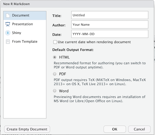
You can stick with the default (HTML output), but give it a title.
Basic components of R Markdown
The initial chunk of text (header) contains instructions for R to specify what kind of document will be created, and the options chosen. You can use the header to give your document a title, author, date, and tell it what type of output you want to produce. In this case, we’re creating an html document.
---
title: "Initial R Markdown document"
author: "Karl Broman"
date: "April 23, 2015"
output: html_document
---
You can delete any of those fields if you don’t want them included. The double-quotes aren’t strictly necessary in this case. They’re mostly needed if you want to include a colon in the title.
RStudio creates the document with some example text to get you started. Note below that there are chunks like
```{r}
summary(cars)
```
These are chunks of R code that will be executed by knitr and replaced
by their results. More on this later.
Markdown
Markdown is a system for writing web pages by marking up the text much as you would in an email rather than writing html code. The marked-up text gets converted to html, replacing the marks with the proper html code.
For now, let’s delete all of the stuff that’s there and write a bit of markdown.
You make things bold using two asterisks, like this: **bold**,
and you make things italics by using underscores, like this:
_italics_.
You can make a bulleted list by writing a list with hyphens or asterisks, like this:
* bold with double-asterisks
* italics with underscores
* code-type font with backticks
or like this:
- bold with double-asterisks
- italics with underscores
- code-type font with backticks
Each will appear as:
- bold with double-asterisks
- italics with underscores
- code-type font with backticks
You can use whatever method you prefer, but be consistent. This maintains the readability of your code.
You can make a numbered list by just using numbers. You can even use the same number over and over if you want:
1. bold with double-asterisks
1. italics with underscores
1. code-type font with backticks
This will appear as:
- bold with double-asterisks
- italics with underscores
- code-type font with backticks
You can make section headers of different sizes by initiating a line
with some number of # symbols:
# Title
## Main section
### Sub-section
#### Sub-sub section
You compile the R Markdown document to an html webpage by clicking the “Knit” button in the upper-left.
Challenge 1
Create a new R Markdown document. Delete all of the R code chunks and write a bit of Markdown (some sections, some italicized text, and an itemized list).
Convert the document to a webpage.
Solution to Challenge 1
In RStudio, select File > New file > R Markdown…
Delete the placeholder text and add the following:
# Introduction ## Background on Data This report uses the *gapminder* dataset, which has columns that include: * country * continent * year * lifeExp * pop * gdpPercap ## Background on MethodsThen click the ‘Knit’ button on the toolbar to generate an html document (webpage).
A bit more Markdown
You can make a hyperlink like this:
[Carpentries Home Page](https://carpentries.org/).
You can include an image file like this: 
You can do subscripts (e.g., F~2~) with F~2~ and superscripts (e.g.,
F^2^) with F^2^.
If you know how to write equations in
LaTeX, you can use $ $ and $$ $$ to insert math equations, like
$E = mc^2$ and
$$y = \mu + \sum_{i=1}^p \beta_i x_i + \epsilon$$
You can review Markdown syntax by navigating to the “Markdown Quick Reference” under the “Help” field in the toolbar at the top of RStudio.
R code chunks
The real power of Markdown comes from mixing markdown with chunks of code. This is R Markdown. When processed, the R code will be executed; if they produce figures, the figures will be inserted in the final document.
The main code chunks look like this:
```{r load_data}
gapminder <- read.csv("gapminder.csv")
```
That is, you place a chunk of R code between ```{r chunk_name}
and ```. You should give each chunk
a unique name, as they will help you to fix errors and, if any graphs are
produced, the file names are based on the name of the code chunk that
produced them. You can create code chunks quickly in RStudio using the shortcuts
Ctrl+Alt+I on Windows and Linux, or Cmd+Option+I on Mac.
Challenge 2
Add code chunks to:
- Load the ggplot2 package
- Read the gapminder data
- Create a plot
Solution to Challenge 2
```{r load-ggplot2} library("ggplot2") ``````{r read-gapminder-data} gapminder <- read.csv("gapminder.csv") ``````{r make-plot} plot(lifeExp ~ year, data = gapminder) ```
How things get compiled
When you press the “Knit” button, the R Markdown document is
processed by knitr and a plain Markdown
document is produced (as well as, potentially, a set of figure files): the R code is executed
and replaced by both the input and the output; if figures are
produced, links to those figures are included.
The Markdown and figure documents are then processed by the tool
pandoc, which converts the Markdown file into an
html file, with the figures embedded.
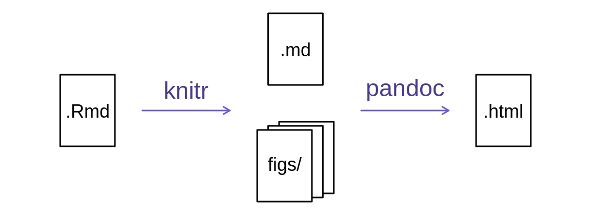
Chunk options
There are a variety of options to affect how the code chunks are treated. Here are some examples:
- Use
echo=FALSEto avoid having the code itself shown. - Use
results="hide"to avoid having any results printed. - Use
eval=FALSEto have the code shown but not evaluated. - Use
warning=FALSEandmessage=FALSEto hide any warnings or messages produced. - Use
fig.heightandfig.widthto control the size of the figures produced (in inches).
So you might write:
```{r load_libraries, echo=FALSE, message=FALSE}
library("dplyr")
library("ggplot2")
```
Often there will be particular options that you’ll want to use repeatedly; for this, you can set global chunk options, like so:
```{r global_options, echo=FALSE}
knitr::opts_chunk$set(fig.path="Figs/", message=FALSE, warning=FALSE,
echo=FALSE, results="hide", fig.width=11)
```
The fig.path option defines where the figures will be saved. The /
here is really important; without it, the figures would be saved in
the standard place but just with names that begin with Figs.
If you have multiple R Markdown files in a common directory, you might
want to use fig.path to define separate prefixes for the figure file
names, like fig.path="Figs/cleaning-" and fig.path="Figs/analysis-".
Challenge 3
Use chunk options to control the size of a figure and to hide the code.
Solution to Challenge 3
```{r echo = FALSE, fig.width = 3} plot(faithful) ```
You can review all of the R chunk options by navigating to
the “R Markdown Cheat Sheet” under the “Cheatsheets” section
of the “Help” field in the toolbar at the top of RStudio.
Inline R code
You can make every number in your report reproducible. Use
`r and ` for an in-line code chunk,
like so: `r round(some_value, 2)`. The code will be
executed and replaced with the value of the result.
Don’t let these in-line chunks get split across lines.
Perhaps precede the paragraph with a larger code chunk that does
calculations and defines variables, with include=FALSE for that larger
chunk (which is the same as echo=FALSE and results="hide").
Rounding can produce differences in output in such situations. You may want
2.0, but round(2.03, 1) will give just 2.
The
myround
function in the R/broman package handles
this.
Challenge 4
Try out a bit of in-line R code.
Solution to Challenge 4
Here’s some inline code to determine that 2 + 2 =
`r 2+2`.
Other output options
You can also convert R Markdown to a PDF or a Word document. Click the
little triangle next to the “Knit” button to get a drop-down
menu. Or you could put pdf_document or word_document in the initial header
of the file.
Tip: Creating PDF documents
Creating .pdf documents may require installation of some extra software. The R package
tinytexprovides some tools to help make this process easier for R users. Withtinytexinstalled, runtinytex::install_tinytex()to install the required software (you’ll only need to do this once) and then when you knit to pdftinytexwill automatically detect and install any additional LaTeX packages that are needed to produce the pdf document. Visit the tinytex website for more information.
Tip: Visual markdown editing in RStudio
RStudio versions 1.4 and later include visual markdown editing mode. In visual editing mode, markdown expressions (like
**bold words**) are transformed to the formatted appearance (bold words) as you type. This mode also includes a toolbar at the top with basic formatting buttons, similar to what you might see in common word processing software programs. You can turn visual editing on and off by pressing thebutton in the top right corner of your R Markdown document.
Resources
- Knitr in a knutshell tutorial
- Dynamic Documents with R and knitr (book)
- R Markdown documentation
- R Markdown cheat sheet
- Getting started with R Markdown
- R Markdown: The Definitive Guide (book by Rstudio team)
- Reproducible Reporting
- The Ecosystem of R Markdown
- Introducing Bookdown
Key Points
Mix reporting written in R Markdown with software written in R.
Specify chunk options to control formatting.
Use
knitrto convert these documents into PDF and other formats.
Writing Good Software (extra)
Overview
Teaching: 15 min
Exercises: 0 minQuestions
How can I write software that other people can use?
Objectives
Describe best practices for writing R and explain the justification for each.
Structure your project folder
Keep your project folder structured, organized and tidy, by creating subfolders for your code files, manuals, data, binaries, output plots, etc. It can be done completely manually, or with the help of RStudio’s New Project functionality, or a designated package, such as ProjectTemplate.
Tip: ProjectTemplate - a possible solution
One way to automate the management of projects is to install the third-party package,
ProjectTemplate. This package will set up an ideal directory structure for project management. This is very useful as it enables you to have your analysis pipeline/workflow organised and structured. Together with the default RStudio project functionality and Git you will be able to keep track of your work as well as be able to share your work with collaborators.
- Install
ProjectTemplate.- Load the library
- Initialise the project:
install.packages("ProjectTemplate") library("ProjectTemplate") create.project("../my_project_2", merge.strategy = "allow.non.conflict")For more information on ProjectTemplate and its functionality visit the home page ProjectTemplate
Make code readable
The most important part of writing code is making it readable and understandable. You want someone else to be able to pick up your code and be able to understand what it does: more often than not this someone will be you 6 months down the line, who will otherwise be cursing past-self.
Documentation: tell us what and why, not how
When you first start out, your comments will often describe what a command does, since you’re still learning yourself and it can help to clarify concepts and remind you later. However, these comments aren’t particularly useful later on when you don’t remember what problem your code is trying to solve. Try to also include comments that tell you why you’re solving a problem, and what problem that is. The how can come after that: it’s an implementation detail you ideally shouldn’t have to worry about.
Keep your code modular
Our recommendation is that you should separate your functions from your analysis
scripts, and store them in a separate file that you source when you open the R
session in your project. This approach is nice because it leaves you with an
uncluttered analysis script, and a repository of useful functions that can be
loaded into any analysis script in your project. It also lets you group related
functions together easily.
Break down problem into bite size pieces
When you first start out, problem solving and function writing can be daunting tasks, and hard to separate from code inexperience. Try to break down your problem into digestible chunks and worry about the implementation details later: keep breaking down the problem into smaller and smaller functions until you reach a point where you can code a solution, and build back up from there.
Know that your code is doing the right thing
Make sure to test your functions!
Don’t repeat yourself
Functions enable easy reuse within a project. If you see blocks of similar lines of code through your project, those are usually candidates for being moved into functions.
If your calculations are performed through a series of functions, then the project becomes more modular and easier to change. This is especially the case for which a particular input always gives a particular output.
Remember to be stylish
Apply consistent style to your code.
Key Points
Keep your project folder structured, organized and tidy.
Document what and why, not how.
Break programs into short single-purpose functions.
Write re-runnable tests.
Don’t repeat yourself.
Be consistent in naming, indentation, and other aspects of style.