Starting with Data

Overview

Teaching: 15 min
Exercises: 5 min

Questions

What is a data.frame?

How can I read a complete csv file into R?

How can I get basic summary information about my dataset?

How are dates represented in R and how can I change the format?

Objectives

Load external data from a .csv file into a data frame.

Install and load packages.

Describe what a data frame is.

Summarize the contents of a data frame.

Use indexing to subset specific portions of data frames.

Describe what a factor is.

Convert between strings and factors.

Reorder and rename factors.

Change how character strings are handled in a data frame.

Format dates.

Loading the Survey Data

library(palmerpenguins)
data(package = 'palmerpenguins')

In this palmerpenguins package, there are two datasets. ‘penguins’ is a simplified version of the raw data, curated for instructional use. Throughout the workshop though, we will also work with the raw data, ‘penguins_raw’.

This dataset is hosted by Palmer Station Antarctica LTER, a member of the Long Term Ecological Research Network. You may also learn more about the research and methodology of this particular dataset: Ecological sexual dimorphism and environmental variability within a community of Antarctic penguins (genus Pygoscelis).

Artwork by @allison_horst

Data Moment: Packages Citation

To get the package’s citation for publication, we can use the citation() function and input the name of the package, "palmerpenguins".
citation("palmerpenguins")
Citation increases reproducibility, which benefits both users and producers. Along with getting the proper credit, citations helps producers keep a bibliographic record of publications and usage which references the cited tools and data.

Because datasets are easier to find with consistent, proper citation of packages and data citation, this practice also encourages reuse of the data for new studies.

This data was originally published in:

Gorman KB, Williams TD, Fraser WR (2014). Ecological sexual dimorphism and environmental variability within a community of Antarctic penguins (genus Pygoscelis). PLoS ONE 9(3):e90081. https://doi.org/10.1371/journal.pone.0090081

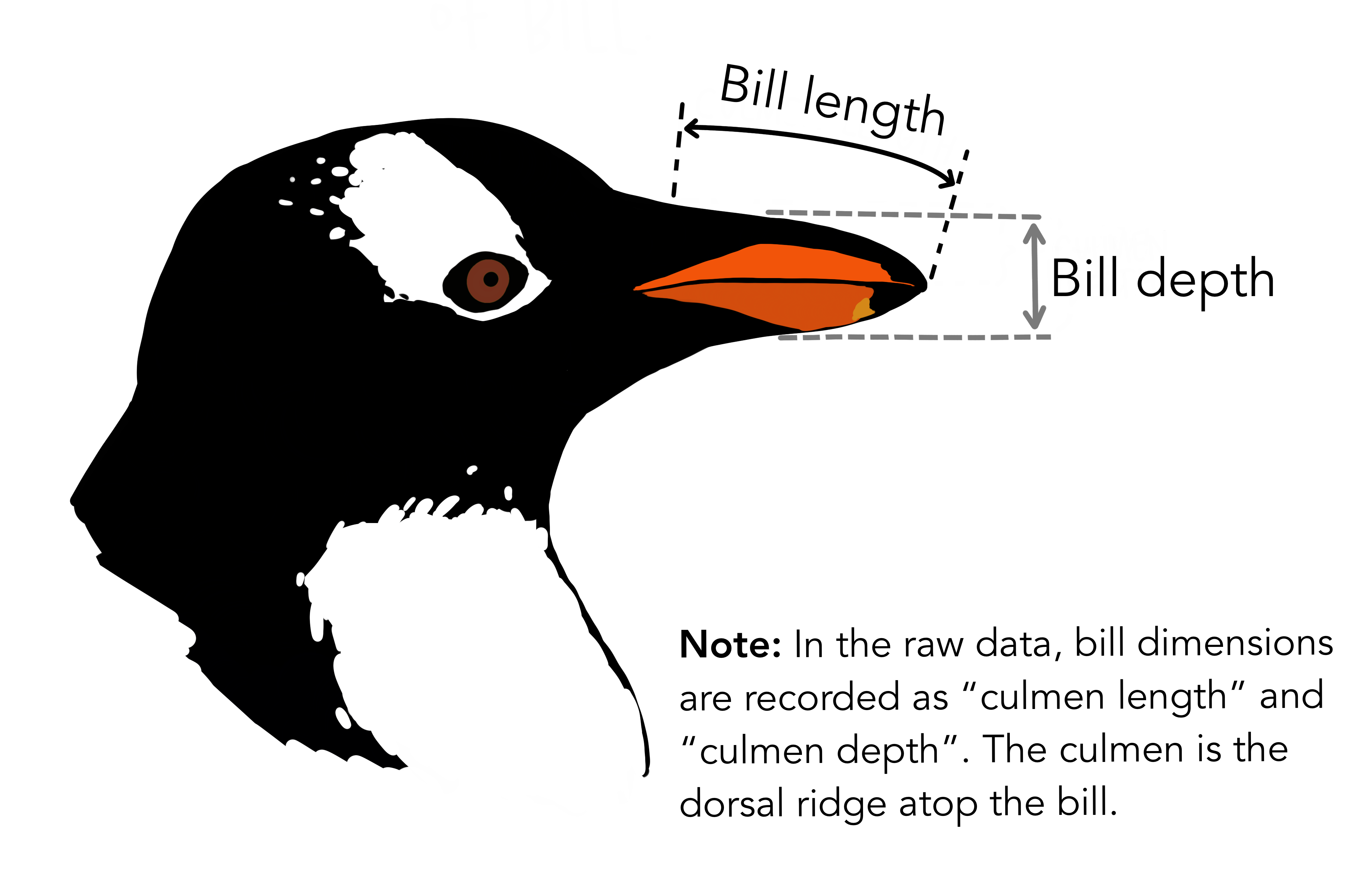
The dataset is stored as a comma separated value (CSV) file. Each row holds information for a date, and the attributes information can be found in the help:

?penguins
?penguins_raw

Artwork by @allison_horst

Reading the Data into R

The file should be downloaded to the destination you specified. R has not yet loaded the data from the file into memory. To do this, we can use the read_csv() function from the tidyverse package.

Packages in R are basically sets of additional functions that let you do more stuff. The functions we’ve been using so far, like round(), sqrt(), or c() come built into R. Packages give you access to additional functions beyond base R. A similar function to read_csv() from the tidyverse package is read.csv() from base R. We don’t have time to cover their differences but notice that the exact spelling determines which function is used. Before you use a package for the first time you need to install it on your machine, and then you should import it in every subsequent R session when you need it.

To install the tidyverse package, we can type install.packages("tidyverse") straight into the console. In fact, it’s better to write this in the console than in our script for any package, as there’s no need to re-install packages every time we run the script. Then, to load the package type:

library(tidyverse)

Now we can use the functions from the tidyverse package. Let’s use read_csv() to read the data into a data frame (we will learn more about data frames later):

penguins <- read.csv(path_to_file("penguins.csv"))

If you have a csv file, you may use read_csv to create an object with it. path_to_file() is not nesessary to use read_csv().

When you execute read_csv on a data file, it looks through the first 1000 rows of each column and guesses its data type. For example, in this dataset, read_csv() reads flipper_length_mm as int (a numeric data type), and species as char. You have the option to specify the data type for a column manually by using the col_types argument in read_csv.

We can see the contents of the first few lines of the data by typing its name: penguins. By default, this will show you as many rows and columns of the data as fit on your screen. If you wanted the first 50 rows, you could type print(penguins, n = 50)

We can also extract the first few lines of this data using the function head():

head(penguins)

  species    island bill_length_mm bill_depth_mm
Adelie Torgersen           39.1          18.7
Adelie Torgersen           39.5          17.4
Adelie Torgersen           40.3          18.0
Adelie Torgersen             NA            NA
Adelie Torgersen           36.7          19.3
Adelie Torgersen           39.3          20.6

 flipper_length_mm body_mass_g    sex year
             181        3750   male 2007
             186        3800 female 2007
             195        3250 female 2007
              NA          NA   <NA> 2007
             193        3450 female 2007
             190        3650   male 2007

Unlike the print() function, head() returns the extracted data. You could use it to assign the first 100 rows of penguins to an object using penguins_sample <- head(penguins, 100). This can be useful if you want to try out complex computations on a subset of your data before you apply them to the whole data set. There is a similar function that lets you extract the last few lines of the data set. It is called (you might have guessed it) tail().

To open the dataset in RStudio’s Data Viewer, use the view() function:

view(penguins)

Note

read_csv() assumes that fields are delineated by commas. However, in several countries, the comma is used as a decimal separator and the semicolon (;) is used as a field delineator. If you want to read in this type of files in R, you can use the read_csv2() function. It behaves like read_csv() but uses different parameters for the decimal and the field separators. There is also the read_tsv() for tab separated data files and read_delim() for less common formats. Check out the help for read_csv() by typing ?read_csv to learn more.

In addition to the above versions of the csv format, you should develop the habits of looking at and recording some parameters of your csv files. For instance, the character encoding, control characters used for line ending, date format (if the date is not split into three variables), and the presence of unexpected newlines are important characteristics of your data files. Those parameters will ease up the import step of your data in R.

What are Data Frames?

When we loaded the data into R, it got stored as an object of class tibble, which is a special kind of data frame (the difference is not important for our purposes, but you can learn more about tibbles here). Data frames are the de facto data structure for most tabular data, and what we use for statistics and plotting. Data frames can be created by hand, but most commonly they are generated by functions like read_csv(); in other words, when importing spreadsheets from your hard drive or the web.

A data frame is the representation of data in the format of a table where the columns are vectors that all have the same length. Because columns are vectors, each column must contain a single type of data (e.g., characters, integers, factors). For example, here is a figure depicting a data frame comprising a numeric, a character, and a logical vector.

We can see this also when inspecting the structure of a data frame with the function str():

str(penguins)

Inspecting Data Frames

We already saw how the functions head() and str() can be useful to check the content and the structure of a data frame. Here is a non-exhaustive list of functions to get a sense of the content/structure of the data. Let’s try them out!

Size:
- dim(penguins) - returns a vector with the number of rows in the first element, and the number of columns as the second element (the dimensions of the object)
- nrow(penguins) - returns the number of rows
- ncol(penguins) - returns the number of columns
Content:
- head(penguins) - shows the first 6 rows
- tail(penguins) - shows the last 6 rows
Names:
- names(penguins) - returns the column names (synonym of colnames() for data.frame objects)
- rownames(penguins) - returns the row names
Summary:
- str(penguins) - structure of the object and information about the class, length and content of each column
- summary(penguins) - summary statistics for each column

Note: most of these functions are “generic”, they can be used on other types of objects besides data.frame.

Challenge

Based on the output of str(penguins), can you answer the following questions?

What is the class of the object penguins?

How many rows and how many columns are in this object?
Solution
 str(penguins)
class: data frame

344 rows, 8 columns

Data Moment: Stuctures

When we look at the stucture of the raw data, we see that it holds 344 observations and 17 variables:

Indexing and Subsetting data frames

Our penguins data frame has rows and columns (it has 2 dimensions). In practice, we may not need the entire data frame; for instance, we may only be interested in a subset of the observations (the rows) or a particular set of variables (the columns). If we want to extract some specific data from it, we need to specify the “coordinates” we want from it. Row numbers come first, followed by column numbers.

# We can extract specific values by specifying row and column indices
# in the format:
# data_frame[row_index, column_index]
# For instance, to extract the first row and column from penguins:
penguins[1, 1]


# First row, fifth column:
penguins[1, 8]   


# We can also use shortcuts to select a number of rows or columns at once
# To select all columns, leave the column index blank
# For instance, to select all columns for the first row:
penguins[1, ]


# The same shortcut works for rows --
# To select the first column across all rows:
penguins[, 1]

# An even shorter way to select first column across all rows:
penguins[1] # No comma!


# To select multiple rows or columns, use vectors!
# To select the first three rows of the 5th and 6th column
penguins[c(1, 2, 3), c(5, 6)]


# We can use the : operator to create those vectors for us:
penguins[1:3, 5:6]


# This is equivalent to head_penguins <- head(penguins)
head_penguins <- penguins[1:6, ]


# As we've seen, when working with tibbles
# subsetting with single square brackets ("[]") always returns a data frame.
# If you want a vector, use double square brackets ("[[]]")
# For instance, to get the first column as a vector:
penguins[[1]]


# To get the first value in our data frame:
penguins[[1, 1]]

: is a special function that creates numeric vectors of integers in increasing or decreasing order, test 1:10 and 10:1 for instance.

You can also exclude certain indices of a data frame using the “-” sign:

penguins[, -1]                 # The whole data frame, except the first column
penguins[-(7:nrow(penguins)), ] # Equivalent to head(penguins)

Data frames can be subset by calling indices (as shown previously), but also by calling their column names directly:

# As before, using single brackets returns a data frame:
penguins["species"]
penguins[, "species"]

# Double brackets returns a vector:
penguins[["species"]]

# We can also use the $ operator with column names instead of double brackets
# This returns a vector:
penguins$species

In RStudio, you can use the autocompletion feature to get the full and correct names of the columns.

Exercise

Create a data.frame (penguins_200) containing only the data in row 200 of the penguins dataset.

Notice how nrow() gave you the number of rows in the data frame?

Use that number to pull out just that last row in the data frame.

Compare that with what you see as the last row using tail() to make sure it’s meeting expectations.

Pull out that last row using nrow() instead of the row number.

Create a new data frame (penguins_last) from that last row.

Use nrow() to extract the row that is in the middle of the data frame. Store the content of this row in an object named penguins_middle.

Combine nrow() with the - notation above to reproduce the behavior of head(penguins), keeping just the first through 6th rows of the penguins dataset.
Solution
## 1.
penguins_200 <- penguins[200, ]
## 2.
# Saving `n_rows` to improve readability and reduce duplication
n_rows <- nrow(penguins)
penguins_last <- penguins[n_rows, ]
## 3.
penguins_middle <-penguins[n_rows/2, ]
## 4.
penguins_head <- penguins[-(7:n_rows), ]

Factors

When we did str(penguins) we saw that several of the columns consist of integers. The columns species, island, sex, however, are of the class character. Arguably, these columns contain categorical data, that is, they can only take on a limited number of values.

R has a special class for working with categorical data, called factor. Factors are very useful and actually contribute to making R particularly well suited to working with data. So we are going to spend a little time introducing them.

Once created, factors can only contain a pre-defined set of values, known as levels. Factors are stored as integers associated with labels and they can be ordered or unordered. While factors look (and often behave) like character vectors, they are actually treated as integer vectors by R. So you need to be very careful when treating them as strings.

When importing a data frame with read_csv(), the columns that contain text are not automatically coerced (=converted) into the factor data type, but once we have loaded the data we can do the conversion using the factor() function:

#create a variable that consists of two levels
low_hi <- c("low", "high", "low", "high")
summary(low_hi)

#using factor conversion
low_hi <- factor(low_hi)

We can see that the conversion has worked by using the summary() function again. This produces a table with the counts for each factor level:

summary(low_hi)

high  low 
   2    2 

R will assign 1 to the level "high" and 2 to the level "low" (because h comes before l, even though the first element in this vector is "low"). You can see this by using the function levels() and you can find the number of levels using nlevels():

levels(low_hi)
nlevels(low_hi)

Sometimes, the order of the factors does not matter, other times you might want to specify the order because it is meaningful (e.g., “low”, “medium”, “high”), it improves your visualization, or it is required by a particular type of analysis. Here, one way to reorder our levels in the class vector would be:

low_hi # current order
low_hi <- factor(class, levels = c("low", "high"))
low_hi # after re-ordering

In R’s memory, these factors are represented by integers (1, 2, 3), but are more informative than integers because factors are self describing: "low", "high" is more descriptive than 1, 2. Which one is “low”? You wouldn’t be able to tell just from the integer data. Factors, on the other hand, have this information built in. It is particularly helpful when there are many levels.

Challenge

Change the columns species and island in the penguins data frame into a factor.

Using the functions you learned before, can you find out… How many rows contain Adelie species?

How many different islands did the research record at?
Solution
penguins$species <- factor(penguins$species)
penguins$island <- factor(penguins$island)

summary(penguins$species)
nlevels(penguins$island)
There are 152 adelie penguines in the species column.

There are 3 unique values in the island column

Converting factors

If you need to convert a factor to a character vector, you use as.character(x).

as.character(low_hi)

In some cases, you may have to convert factors where the levels appear as numbers (such as concentration levels or years) to a numeric vector. For instance, in one part of your analysis the years might need to be encoded as factors (e.g., comparing average weights across years) but in another part of your analysis they may need to be stored as numeric values (e.g., doing math operations on the years). This conversion from factor to numeric is a little trickier. The as.numeric() function returns the index values of the factor, not its levels, so it will result in an entirely new (and unwanted in this case) set of numbers. One method to avoid this is to convert factors to characters, and then to numbers.

Another method is to use the levels() function. Compare:

year_fct <- factor(c(1991, 1992, 1993, 1994, 1995))
as.numeric(year_fct)               # Wrong! And there is no warning...
as.numeric(as.character(year_fct)) # Works...
as.numeric(levels(year_fct))[year_fct]    # The recommended way.

Notice that in the levels() approach, three important steps occur:

We obtain all the factor levels using levels(year_fct)
We convert these levels to numeric values using as.numeric(levels(year_fct))
We then access these numeric values using the underlying integers of the vector year_fct inside the square brackets

as.numeric(year_fct)  # Wrong! And there is no warning...

3 1 2 4 5

as.numeric(as.character(year_fct))  # Works...

[1] 1991 1992 1993 1994 1995

as.numeric(levels(year_fct))[year_fct]  # The recommended way.

[1] 1991 1992 1993 1994 1995

Notice that in the recommended levels() approach, three important steps occur:

We obtain all the factor levels using levels(year_fct)
We convert these levels to numeric values using as.numeric(levels(year_fct))
We then access these numeric values using the underlying integers of the vector year_fct inside the square brackets

Renaming factors

When your data is stored as a factor, you can get a quick glance at the number of observations represented by each factor level. Let’s look at the number of males and females observed:

penguins$sex <- factor(penguins$sex)
plot(penguins$sex)

However, as we saw when we used summary(surveys$sex), there are 11 individuals for which the sex information hasn’t been recorded. To show them in the plot, we can turn the missing values into a factor level with the addNA() function. We will also have to give the new factor level a label. We are going to work with a copy of the sex column, so we’re not modifying the working copy of the data frame:

sex <- surveys$sex
levels(sex)

sex <- addNA(sex)
levels(sex)

head(sex)

levels(sex)[3] <- "undetermined"
levels(sex)

Now we can plot the data again, using plot(sex).

Challenge:

Rename “F” and “M” to “female” and “male” respectively. Now that we have renamed the factor level to “undetermined”, can you recreate the barplot such that “undetermined” is first (before “female”)?
Solution
levels(sex)[1:2] <- c("F", "M")
sex <- factor(sex, levels = c("undetermined", "female", "male"))
plot(sex)

Challenge

We have seen how data frames are created when using the read.csv(), but they can also be created by hand with the data.frame() function. There are a few mistakes in this hand-crafted data.frame, can you spot and fix them? Don’t hesitate to experiment!

 animal_data <- data.frame(animal = c("dog", "cat", "sea cucumber", "sea urchin"),
                           feel = c("furry", "squishy", "spiny"),
                           weight = c(45, 8 1.1, 0.8))

 ## Challenge:
 ##  There are a few mistakes in this hand-crafted `data.frame`,
 ##  can you spot and fix them? Don't hesitate to experiment!
 animal_data <- data.frame(animal = c(dog, cat, sea cucumber, sea urchin),
                           feel = c("furry", "squishy", "spiny"),
                           weight = c(45, 8 1.1, 0.8))

Can you predict the class for each of the columns in the following example? Check your guesses using str(country_climate):

Are they what you expected? Why? Why not?
What would have been different if we had added stringsAsFactors = FALSE to this call?
What would you need to change to ensure that each column had the accurate data type?

 country_climate <- data.frame(
        country = c("Canada", "Panama", "South Africa", "Australia"),
        climate = c("cold", "hot", "temperate", "hot/temperate"),
        temperature = c(10, 30, 18, "15"),
        northern_hemisphere = c(TRUE, TRUE, FALSE, "FALSE"),
        has_kangaroo = c(FALSE, FALSE, FALSE, 1)
        )

## Challenge:
##   Can you predict the class for each of the columns in the following
##   example?
##   Check your guesses using `str(country_climate)`:
##   * Are they what you expected? Why? why not?
##   * What would have been different if we had added `stringsAsFactors = FALSE`
##     to this call?
##   * What would you need to change to ensure that each column had the
##     accurate data type?
country_climate <- data.frame(country = c("Canada", "Panama", "South Africa", "Australia"),
                               climate = c("cold", "hot", "temperate", "hot/temperate"),
                               temperature = c(10, 30, 18, "15"),
                               northern_hemisphere = c(TRUE, TRUE, FALSE, "FALSE"),
                               has_kangaroo = c(FALSE, FALSE, FALSE, 1))

Solution

missing quotations around the names of the animals

missing one entry in the “feel” column (probably for one of the furry animals)

missing one comma in the weight column

country, climate, temperature, and northern_hemisphere are factors; has_kangaroo is numeric.

using stringsAsFactors=FALSE would have made them character instead of factors

removing the quotes in temperature, northern_hemisphere, and replacing 1 by TRUE in the has_kangaroo column would probably what was originally intended.

Formatting Dates

A common issue that new (and experienced!) R users have is converting date and time information into a variable that is suitable for analyses. One way to store date information is to store each component of the date in a separate column. Using str(), we can confirm that our data frame does indeed have a separate column for day, month, and year, and that each of these columns contains integer values.

str(penguins)

We are going to use the ymd() function from the package lubridate (which belongs to the tidyverse; learn more here). lubridate gets installed as part as the tidyverse installation. When you load the tidyverse (library(tidyverse)), the core packages (the packages used in most data analyses) get loaded. lubridate however does not belong to the core tidyverse, so you have to load it explicitly with library(lubridate)

Start by loading the required package:

library(lubridate)

The lubridate package has many useful functions for working with dates. These can help you extract dates from different string representations, convert between timezones, calculate time differences and more. You can find an overview of them in the lubridate cheat sheet.

Let’s create an object and inspect the structure:

str("2022-01-01")

chr "2022-01-01"

Note that R reads this as a character. Now let’s paste the year, month, and day separately - we get the same result:

# sep indicates the character to use to separate each component
str(paste("2022", "01", "01", sep = "-"))

chr "2022-1-1"

Here we will use the function ymd(), which takes a vector representing year, month, and day, and converts it to a Date vector. Date is a class of data recognized by R as being a date and can be manipulated as such. The argument that the function requires is flexible, but, as a best practice, is a character vector formatted as “YYYY-MM-DD”.

my_date <- ymd(paste("2022", "01", "01", sep = "-"))
str(my_date)

Now lets look at the penguines_raw dataset and extract the column Date Egg.

egg_dates <- penguins_raw$`Date Egg`
str(egg_dates)

Let’s extract our Date Egg column and inspect the structure.

What is “Date Egg”?
?penguins_raw

We are able to pull the year, month, and day from the date values:

egg_yr <- year(egg_dates)
egg_mo <- month(egg_dates)
egg_day <- day(egg_dates)

When we imported the data in R, read_csv() recognized that this column contained date information. We can use the day(), month() and year() functions to extract this information from the date, and create new columns in our data frame to store it:

# we can create dataframes
egg_dates_df <- data.frame(year = egg_yr, month = egg_mo, day = egg_day)

egg_dates_df

    year month day
 2007    11  11
 2007    11  11
 2007    11  16
 2007    11  16
 2007    11  16
...

These character vectors can be used as the argument for ymd():

ymd(paste(egg_dates_df$year, egg_dates_df$month, egg_dates_df$day, sep = "-"))

In our example above, the Date Egg column was read in correctly as a Date variable but generally that is not the case. Date columns are often read in as character variables and one can use the as_date() function to convert them to the appropriate Date/POSIXctformat.

Let’s say we have a vector of dates in character format:

char_dates <- c("01/01/2020", "02/02/2020", "03/03/2020")
str(char_dates)

chr [1:3] "01/01/2020" "02/02/2020" "03/03/2020"

We can convert this vector to dates as :

as_date(char_dates, format = "%m/%d/%Y")

[1] "2012-07-31" "2014-08-09" "2016-04-30"

Argument format tells the function the order to parse the characters and identify the month, day and year. The format above is the equivalent of mm/dd/yyyy. A wrong format can lead to parsing errors or incorrect results.

For example, observe what happens when we use a lower case y instead of upper case Y for the year.

as_date(char_dates, format = "%m/%d/%y")

[1] "2020-01-01" "2020-02-02" "2020-03-03"

Here, the %y part of the format stands for a two-digit year instead of a four-digit year, and this leads to parsing errors.

Or in the following example, observe what happens when the month and day elements of the format are switched.

as_date(char_dates, format = "%d/%m/%y")

[1] NA           "2020-09-08" NA

Since there is no month numbered 30 or 31, the first and third dates cannot be parsed.

We can also use functions ymd(), mdy() or dmy() to convert character variables to date.

mdy(char_dates)

Data Package Citation

Horst AM, Hill AP, Gorman KB (2020). palmerpenguins: Palmer Archipelago (Antarctica) penguin data. R package version 0.1.0. https://allisonhorst.github.io/palmerpenguins/

Key Points

Use read_csv to read tabular data in R.

Use factors to represent categorical data in R.

previous episode

Data Analysis and Visualization in R (for Ecologists)

next episode

Starting with Data

Overview

Loading the Survey Data

Data Moment: Packages Citation

Reading the Data into R

Note

What are Data Frames?

Inspecting Data Frames

Challenge

Solution

Data Moment: Stuctures

Indexing and Subsetting data frames

Exercise

Solution

Factors

Challenge

Solution

Converting factors

Renaming factors

Challenge:

Solution

Challenge

Solution

Formatting Dates

What is “Date Egg”?

Data Package Citation

Key Points

previous episode

next episode