Getting started with Quarto

Estimated time: 45 minutes

Instructor Note

• This is an optional lesson intended to introduce learners to Quarto.
• While it is listed after the core lessons, some instructors may prefer to teach it early in the workshop, depending on the audience.

Overview

Questions

• What is Quarto?
• How can I integrate my R code with text and plots?
• How can I convert .qmd files to .html?

Objectives

• Create a .qmd document containing R code, text, and plots
• Create a YAML header to control the output
• Understand the basic syntax of Quarto
• Customize code chunks to control formatting
• Use code chunks and in-line code to create dynamic, reproducible documents

Quarto

---

Quarto is an open-source scientific and technical publishing system for integrating code, text, figures, citations, etc., to produce elegantly formatted output as documents, web pages, blog posts, books and more.

If you’ve heard of or used R Markdown, Quarto is closely related to it, but with the advantage of supporting multi-language projects, more built-in output formats, and options for customizing and creating dynamic content natively in RStudio instead of relying on external packages.

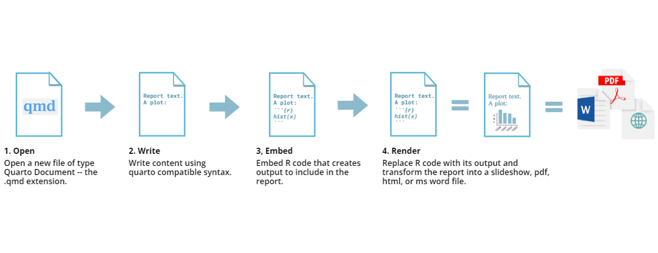
Quarto allows you to produce research reports with minimal reproducibility friction. It provides an environment where you can write your complete analysis. It weaves your text, figures, code, and citations into a single document. The following sections cover examples of using Quarto to explore data with collaborators and communicate your science. Documents created with Quarto can be readily converted to multiple static and dynamic output formats, including PDF (.pdf), Word (.docx), and HTML (.html).

Quarto comes pre-installed with your RStudio IDE (v2022.07 and later), so there’s no need for anything before we can move on.

Creating a Quarto file

---

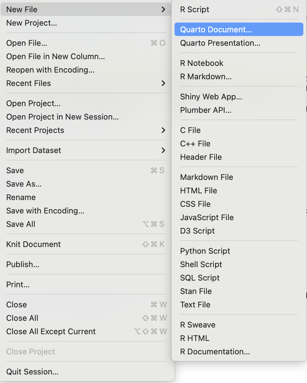
To create a new Quarto document in RStudio, click File -> New File -> Quarto Document:

Then click on ‘Create Empty Document’. Typically, you could enter the title of your document, your name (Author), and select the type of output, but we will learn how to start from a blank document.

Basic components of Quarto

---

To control the output, a YAML (YAML Ain’t Markup Language) header is needed:

---
title: "Untitled"
format: html
editor: visual
---

The header is defined by the three hyphens at the beginning (---) and the three hyphens at the end (---).

In the YAML, the only required field is the format:, which specifies the type of output you want. This can be an html, a pdf, or a word. We will start with an HTML document and discuss the other options later.

After the header, to begin the body of the document, you start typing after the end of the YAML header (i.e., after the second ---).

While we will stick to the basics, it is important to note that Quarto provides a rich set of YAML metadata keys to describe front matter details and configuration settings to customize how your document will render. Even though we won’t be able to cover those today, here is an an example that can inspire you to explore it further:

---
title: "Toward a Unified Theory of High-Energy Metaphysics: Silly String Theory"
date: 2008-02-29
author:
  - name: Josiah Carberry
    id: jc
    orcid: 0000-0002-1825-0097
    email: josiah@psychoceramics.org
    affiliation:
      - name: Brown University
        city: Providence
        state: RI
        url: www.brown.edu
abstract: >
  The characteristic theme of the works of Stone is
  the bridge between culture and society. ...
keywords:
  - Metaphysics
  - String Theory
license: "CC BY"
copyright:
  holder: Josiah Carberry
  year: 2008
citation:
  container-title: Journal of Psychoceramics
  volume: 1
  issue: 1
  doi: 10.5555/12345678
funding: "The author received no specific funding for this work."
---

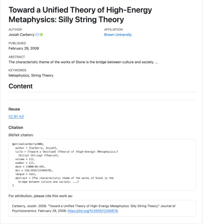
The image below shows how this Quarto document would look as an html output:

Markdown syntax

---

Even though RStudio supports the visual mode, with which you can accomplish most formatting without syntax typing, it is worth understanding its basics.

Markdown is a popular markup language that allows you to add formatting elements to text, such as bold, italics, and code. The formatting will not be immediately visible in a markdown (.md) document like in Word. Instead, you add Markdown syntax to the text, which can then be converted to various other files that can translate the Markdown syntax. Markdown is helpful because it is lightweight, flexible, and platform-independent.

First, let’s create a heading! A # in front of the text indicates to Markdown that this text is a heading. Adding more #s make the heading smaller, i.e., one # is a first-level heading, two ##s is a second-level heading, etc., up to the 6th level heading.

# Title
## Section
### Sub-section
#### Sub-sub section
##### Sub-sub-sub section
###### Sub-sub-sub-sub section

Ensure only to use a level if the one above is also in use.

Since we have already defined our title in the YAML header, we will use a section heading to create an Introduction section.

## Introduction

You can make things bold by surrounding the word with a double asterisks, **bold**, or double underscores, __bold__; and italicize using single asterisks, *italics*, or single underscores, _italics_.

You can also combine bold and italics to write something really important with triple-asterisks, ***really***, or underscores, ___really___; and, if you’re feeling bold (pun intended), you can also use a combination of asterisks and underscores, **_really_**, really.

To create code-type font, surround the word with backticks, `code-type`.

Now that we’ve learned a couple of things, it might be useful to implement them:

## Introduction

This report uses the **tidyverse** package along with the *surveys_complete_77_89.csv* dataset,
which has columns that include:

Then, we can create a list of the variables using the -, +, or * keys.

## Introduction

This report uses the **tidyverse** package along with the *surveys_complete_77_89.csv* dataset,
which has columns that include:

- record_id
- month
- day
- year
- plot_id
- species_id

You can also create an ordered list using numbers:

1. record_id
2. month
3. day
4. year
5. plot_id
6. species_id

And nested items by tab-indenting:

- record_id
  + unique case number
- month
  + month case was recorded
- day
  + month case was recorded
- year
  + year was recorded
- plot_id
  + unique plot ID
- species_id
  + species alpha code

For more Markdown syntax, see the following reference guide.

Now we can render the document into HTML by clicking the Render button at the top of the Source pane (top left), or use the keyboard shortcut Ctrl+Shift+K on Windows and Linux, and Cmd+Shift+K on Mac. If you haven’t saved the document yet, you will be prompted to do so when you Render for the first time.

Writing a Quarto report

---

Now, we will add some R code from previous episodes, meaning we need to ensure ggplot2 and dplyr are loaded. It is not enough to load tidyverse from the console, we will need to load it within our Quarto document. The same applies to our data. To load these, we will need to create a ‘code chunk’ at the top of our document (below the YAML header).

A code chunk can be inserted by clicking Code > Insert Chunk, or by using the keyboard shortcuts Ctrl+Alt+I on Windows and Linux, and Cmd+Option+I on Mac.

The syntax of a code chunk is:

MARKDOWN

```{r}

"Here is where you place the R code you want to run."

```

In Quarto, you can label a code chunk by adding a label:

MARKDOWN

```{r}
#| label: testing

"Here is where you place the R code you want to run."

```

A Quarto document knows that this text is not part of the report from the ``` that begins and ends the chunk. It also knows that the code inside of the chunk is R code from the r inside of the curly braces ({}). After the r, you can add a name for the code chunk. As mentioned, Quarto is multi-language, and you may enter other programming languages for specific code chunks if desired. However, this workshop focuses on R, so let’s stick to that.

Naming a chunk is optional but recommended for easier referencing and future updates. Please keep in mind that each chunk name must be unique and can only include alphanumeric characters and hyphens (-).

To load ggplot2 and dplyr and our surveys_complete_77_89.csv file, we will insert a chunk and call it ‘genus-comp’.

MARKDOWN

```{r}
#| label: genus-comp
# Load necessary packages
library(tidyverse)

# Load the dataset
surveys <- read_csv("data/cleaned/surveys_complete_77_89.csv")

# Count occurrences of Dipodomys and Onychomys by year
occurrences_by_year <- surveys %>%
  filter(genus %in% c("Dipodomys", "Onychomys")) %>%
  group_by(year, genus) %>%
  summarize(count = n(), .groups = 'drop')

# Plotting the data
ggplot(occurrences_by_year, aes(x = year, y = count, color = genus, group = genus)) +
  geom_line() +
  geom_point() +
  labs(title = "Dipodomys vs. Onychomys by Year",
       x = "Year",
       y = "Occurrences") +
  theme_minimal() +
  scale_x_continuous(breaks = unique(occurrences_by_year$year))

```

You don’t need to Render your entire document whenever you want to view how the code you are currently working on is rendering. While this might not be an issue for shorter documents, it can be time-consuming with many code chunks when you want to check the output of a specific block. In such cases, you can run the code chunk by clicking the green triangle in the top right corner, or by using the keyboard shortcuts: Ctrl+Alt+C on Windows and Linux, or Cmd+Option+C on Mac.

Run the code chunk to make sure you get the desired output.

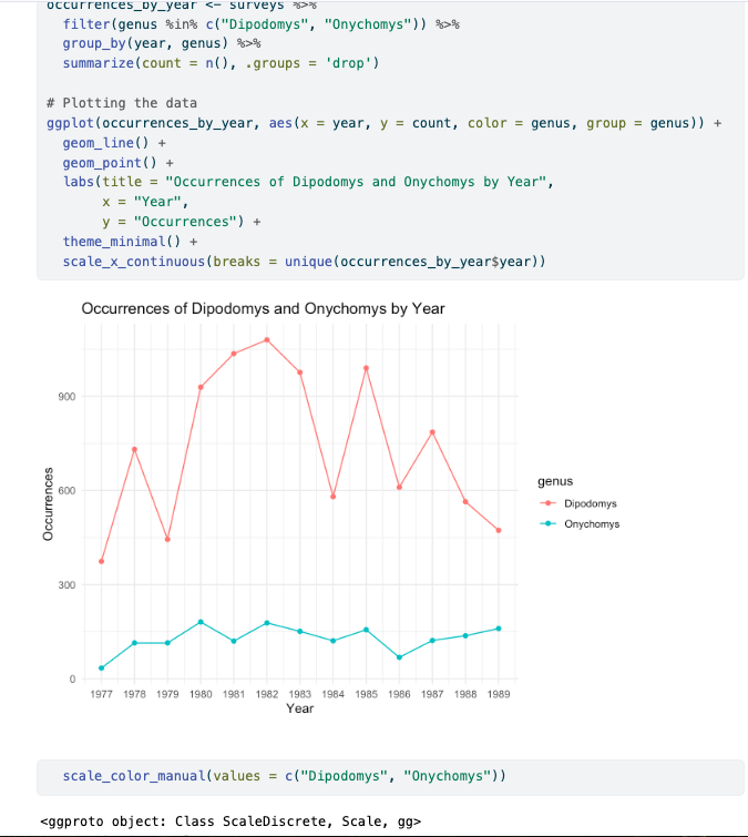
We generated a rendered plot, but it includes many unnecessary elements that we may not want in our report. Let’s explore how we can enhance it.

More on customizing chunk outputs

---

There are several code and cell output options that you can use to customize how things will look in your rendered .qmd document. Below are a few of the most commonly used:

Option	Options	Output
eval	TRUE or FALSE	Whether or not the code within the code chunk should be run.
echo	TRUE or FALSE	Choose to show your code chunk in the output document. echo = TRUE will show the code chunk.
include	TRUE or FALSE	Choose if the output of a code chunk should be included in the document. FALSE means that your code will run, but will not show up in the document.
warning	TRUE or FALSE	Whether or not you want your output document to display potential warning messages produced by your code.
message	TRUE or FALSE	Whether or not you want your output document to display potential messages produced by your code.
results	markup, asis, HOLD, or FALSE	How to display text results. Note that this option only applies to normal text output (not warnings, messages, or errors).

Explore these and other options Code Cells: Knitr

More about custom code chunks

• The default settings for the above chunk options are all TRUE.
• The default settings can be modified per chunk, or across the whole .qmd document using the execution options at the YAML level.
• There is also an option to apply global options to all .qmd files contained in a quarto project using the _quarto.yml file configuration. But that is an advanced setup we encourage you to explore with more time.

Exercise

Which option would I need to apply to the `genus-comp` example to not render the extra content from the plot?

Show me the solution

#| echo: FALSE

#| warning: FALSE

#| message: FALSE

#| results: FALSE

Exercise

Copy the code in the R script used to generate the blue graph in early episodes below. Create a code chunk in your .qmd document, and play around with the different options in the chunk with the code for the table, and Render the document or the code chunk to see what each option does to the output.

What happens if you use eval = FALSE and echo = FALSE? What is the difference between this and include = FALSE?

R

ggplot(data = complete_old, mapping = aes(x = weight, y = hindfoot_length)) +
  geom_point(alpha = 0.2, color = "blue")`

Show me the solution

Create a chunk with {r eval = FALSE, echo = FALSE}, then create another chunk with {r include = FALSE} to compare. eval = FALSE and echo = FALSE will neither run the code in the chunk nor show the code in the rendered document. The code chunk doesn’t exist in the rendered document, as it was never run. On the other hand, include = FALSE will run the code and store the output for later use.

In-line R code

---

We’ve discussed code chunks and how to include them in a QMD document, but what if you want to integrate inline R code to present descriptive statistics in your paper? Using inline code can enhance your narrative by allowing dynamic values to appear alongside your text. Instead of manually typing static values, you can call them directly from your dataset. If your data changes, the values will automatically update, ensuring your results are always current.

To use in-line R-code, we use the same backticks that we used in the Markdown section, with an r to specify that we are generating R-code. The difference between in-line code and a code chunk is the number of backticks. In-line R code uses one backtick (`r`), whereas code chunks use three backticks (```r```).

The best way to use in-line R code, is to minimize the amount of code you need to produce the in-line output by preparing the output in code chunks. Let’s say we’re interested in presenting our dataset’s average number of rodents.

Now, we can make an informative statement as an in-line R-code. For example:

Our dataset includes `{r} nrow(surveys)` cases.

becomes…

Our dataset includes 16878 cases.

Because we are using in-line R code instead of the actual values, we have created a dynamic document that will automatically update if we change the dataset and/or code chunks. Cool, right?

Exercise

Create an in-line code to represent the average weight for the sample:

“Our sample includes 16878 cases, with an average weight of ?

Show me the solution

…, with an average weight weight of `{r} mean(as.integer(surveys$hindfoot_length), na.rm = TRUE)` millimeters.

becomes…

…, with an average hindfoot length of 31.9821138 millimeters.

If you feel inspired, you may also round it up 31.98

…, with an average weight weight of `{r} round(mean(as.integer(surveys$hindfoot_length), na.rm = TRUE)` millimeters.

becomes…

…, with an average hindfoot length of 31.98

Other output options

---

You can convert Quarto to other formats. Quarto documents are currently supported as HTML (html), PDF (pdf), MS Word (docx), OpenOffice (odt) and ePub (epub). You may describe the desired output in the YAML.

---
title: "My Awesome Report"
author: "Your name"
output: docx
---

Alternatively, you can specify the use of a format on the command line:

BASH

quarto render document.qmd --to docx

Note: Creating PDF documents

In order to create PDFs you will need to install a recent distribution of TeX. We recommend the use of TinyTeX (which is based on TexLive), which you can install with the following command in the terminal:

BASH

quarto install tinytex

Note: Inserting citations into a Quarto file

It is possible to insert citations into a Quarto file using the editor toolbar. The editor toolbar includes formatting buttons commonly seen in text editors (e.g., bold and italic). The toolbar is accessible by using the settings drop-down menu (next to the ‘Render’ drop-down menu) to select ‘Use Visual Editor’, which is also accessible through the shortcut ‘Crtl+Shift+F4’. From here, click ‘Insert’ allows ‘Citation’ to be selected (shortcut: ‘Crtl+Shift+F8’). For example, searching ‘10.1007/978-3-319-24277-4’ in ‘From DOI’ and inserting will provide the citation for ggplot2 [@wickham2016]. This will also save the citation(s) in ‘references.bib’ in the current working directory. Visit the R Studio website for more information. Tip: You may also change citation styles automatically (see: https://quarto.org/docs/authoring/citations.html).

Resources

---

• Markdown Basics
• Introduction to Reproducible Publications with RStudio

Key Points

• Quarto is useful for creating reproducible documents combining text, code and figures.
• Specify chunk options to control the formatting of the output document.