Reproject Raster Data
Overview
Teaching: 10 min
Exercises: 10 minQuestions
How do I work with raster data sets that are in different projections?
Objectives
Reproject a raster in R.
Things You’ll Need To Complete This Episode
See the lesson homepage for detailed information about the software, data, and other prerequisites you will need to work through the examples in this episode.
Sometimes we encounter raster datasets that do not “line up” when plotted or
analyzed. Rasters that don’t line up are most often in different Coordinate
Reference Systems (CRS). This episode explains how to deal with rasters in different, known CRSs. It
will walk though reprojecting rasters in R using the projectRaster()
function in the raster package.
Raster Projection in R
In the Plot Raster Data in R episode, we learned how to layer a raster file on top of a hillshade for a nice looking basemap. In that episode, all of our data were in the same CRS. What happens when things don’t line up?
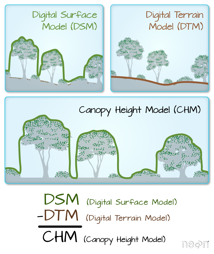
For this episode, we will be working with the Harvard Forest Digital Terrain Model data. This differs from the surface model data we’ve been working with so far in that the digital surface model (DSM) includes the tops of trees, while the digital terrain model (DTM) shows the ground level.
We’ll be looking at another model (the canopy height model) in
a later episode and will see how to calculate the CHM from the
DSM and DTM. Here, we will create a map of the Harvard Forest Digital
Terrain Model
(DTM_HARV) draped or layered on top of the hillshade (DTM_hill_HARV).
The hillshade layer maps the terrain using light and shadow to create a 3D-looking image,
based on a hypothetical illumination of the ground level.
First, we need to import the DTM and DTM hillshade data.
DTM_HARV <- raster("data/NEON-DS-Airborne-Remote-Sensing/HARV/DTM/HARV_dtmCrop.tif")

DTM_hill_HARV <- raster("data/NEON-DS-Airborne-Remote-Sensing/HARV/DTM/HARV_DTMhill_WGS84.tif")
Next, we will convert each of these datasets to a dataframe for
plotting with ggplot.
DTM_HARV_df <- as.data.frame(DTM_HARV, xy = TRUE)

DTM_hill_HARV_df <- as.data.frame(DTM_hill_HARV, xy = TRUE)
Now we can create a map of the DTM layered over the hillshade.
ggplot() +
     geom_raster(data = DTM_HARV_df ,
                 aes(x = x, y = y,
                  fill = HARV_dtmCrop)) +
     geom_raster(data = DTM_hill_HARV_df,
                 aes(x = x, y = y,
                   alpha = HARV_DTMhill_WGS84)) +
     scale_fill_gradientn(name = "Elevation", colors = terrain.colors(10)) +
     coord_quickmap()

Our results are curious - neither the Digital Terrain Model (DTM_HARV_df)
nor the DTM Hillshade (DTM_hill_HARV_df) plotted.
Let’s try to
plot the DTM on its own to make sure there are data there.
ggplot() +
geom_raster(data = DTM_HARV_df,
    aes(x = x, y = y,
    fill = HARV_dtmCrop)) +
scale_fill_gradientn(name = "Elevation", colors = terrain.colors(10)) +
coord_quickmap()

Our DTM seems to contain data and plots just fine.
Next we plot the DTM Hillshade on its own to see whether everything is OK.
ggplot() +
geom_raster(data = DTM_hill_HARV_df,
    aes(x = x, y = y,
    alpha = HARV_DTMhill_WGS84)) +
    coord_quickmap()

If we look at the axes, we can see that the projections of the two rasters are different.
When this is the case, ggplot won’t render the image. It won’t even
throw an error message to tell you something has gone wrong. We can look at Coordinate Reference Systems (CRSs) of the DTM and
the hillshade data to see how they differ.
Exercise
View the CRS for each of these two datasets. What projection does each use?
Solution
Because the two rasters are in different CRSs, they don’t line up when plotted
in R. We need to reproject (or change the projection of) DTM_hill_HARV into the UTM CRS. Alternatively,
we could reproject DTM_HARV into WGS84.
Reproject Rasters
We can use the projectRaster() function to reproject a raster into a new CRS.
Keep in mind that reprojection only works when you first have a defined CRS
for the raster object that you want to reproject. It cannot be used if no
CRS is defined. Lucky for us, the DTM_hill_HARV has a defined CRS.
Data Tip
When we reproject a raster, we move it from one “grid” to another. Thus, we are modifying the data! Keep this in mind as we work with raster data.
To use the projectRaster() function, we need to define two things:
- the object we want to reproject and
- the CRS that we want to reproject it to.
The syntax is projectRaster(RasterObject, crs = CRSToReprojectTo)
We want the CRS of our hillshade to match the DTM_HARV raster. We can thus
assign the CRS of our DTM_HARV to our hillshade within the projectRaster()
function as follows: crs = crs(DTM_HARV).
Note that we are using the projectRaster() function on the raster object,
not the data.frame() we use for plotting with ggplot.
First we will reproject our DTM_hill_HARV raster data to match the DTM_HARV raster CRS:
DTM_hill_UTMZ18N_HARV <- projectRaster(DTM_hill_HARV,
crs = crs(DTM_HARV))
Now we can compare the CRS of our original DTM hillshade and our new DTM hillshade, to see how they are different.
crs(DTM_hill_UTMZ18N_HARV)
CRS arguments:
 +proj=utm +zone=18 +datum=WGS84 +units=m +no_defs
crs(DTM_hill_HARV)
CRS arguments: +proj=longlat +datum=WGS84 +no_defs
We can also compare the extent of the two objects.
extent(DTM_hill_UTMZ18N_HARV)
class      : Extent
xmin       : 731397.3
xmax       : 733205.3
ymin       : 4712403
ymax       : 4713907
extent(DTM_hill_HARV)
class      : Extent
xmin       : -72.18192
xmax       : -72.16061
ymin       : 42.52941
ymax       : 42.54234
Notice in the output above that the crs() of DTM_hill_UTMZ18N_HARV is now
UTM. However, the extent values of DTM_hillUTMZ18N_HARV are different from
DTM_hill_HARV.
Challenge: Extent Change with CRS Change
Why do you think the two extents differ?
Answers
Deal with Raster Resolution
Let’s next have a look at the resolution of our reprojected hillshade versus our original data.
res(DTM_hill_UTMZ18N_HARV)
[1] 1.000 0.998
res(DTM_HARV)
[1] 1 1
These two resolutions are different, but they’re representing the same data. We can tell R to force our
newly reprojected raster to be 1m x 1m resolution by adding a line of code
res=1 within the projectRaster() function. In the example below, we ensure a resolution match by using res(DTM_HARV) as a variable.
  DTM_hill_UTMZ18N_HARV <- projectRaster(DTM_hill_HARV,
                                         crs = crs(DTM_HARV),
                                         res = res(DTM_HARV))
Now both our resolutions and our CRSs match, so we can plot these two data sets together. Let’s double-check our resolution to be sure:
res(DTM_hill_UTMZ18N_HARV)
[1] 1 1
res(DTM_HARV)
[1] 1 1
For plotting with ggplot(), we will need to create a dataframe from our newly reprojected raster.
DTM_hill_HARV_2_df <- as.data.frame(DTM_hill_UTMZ18N_HARV, xy = TRUE)
We can now create a plot of this data.
ggplot() +
     geom_raster(data = DTM_HARV_df ,
                 aes(x = x, y = y,
                  fill = HARV_dtmCrop)) +
     geom_raster(data = DTM_hill_HARV_2_df,
                 aes(x = x, y = y,
                   alpha = HARV_DTMhill_WGS84)) +
     scale_fill_gradientn(name = "Elevation", colors = terrain.colors(10)) +
     coord_quickmap()

We have now successfully draped the Digital Terrain Model on top of our hillshade to produce a nice looking, textured map!
Challenge: Reproject, then Plot a Digital Terrain Model
Create a map of the San Joaquin Experimental Range field site using the
SJER_DSMhill_WGS84.tifandSJER_dsmCrop.tiffiles.Reproject the data as necessary to make things line up!
Answers
If you completed the San Joaquin plotting challenge in the Plot Raster Data in R episode, how does the map you just created compare to that map?
Answers

Key Points
In order to plot two raster data sets together, they must be in the same CRS.
Use the
projectRaster()function to convert between CRSs.